StationaryCovarianceModelFactory¶

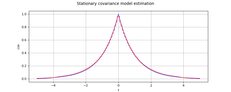
(Source code, png, hires.png, pdf)

class StationaryCovarianceModelFactory(*args)¶

Estimation of the covariance model of a stationary process.

Refer to Estimation of a stationary covariance model.

Parameters

spectralModelFactorySpectralModelFactory

The spectral model factory.

By default, it is the Welch factory model.

Notes

We consider $X: \Omega \times \cD \rightarrow \Rset^d$ be a multivariate process of dimension d where $\cD \in \Rset^n$ . We only treat here the case where the domain is of dimension 1: $\cD \in \Rset$ ( $n=1$ ). We denote $(\vect{t}_0, \dots, \vect{t}_{N-1})$ the vertices of the mesh $\cM \in \cD$ which is a time grid supposed regular.

X is supposed to be a stationary second order process with zero mean. We note its covariance function $C^{stat}: \cD \rightarrow \mathcal{M}_{d \times d}(\Rset)$ , defined by $C^{stat}(\tau)=\Expect{X_s\Tr{X_{s+\tau}}}$ for all $s\in \cD$ .

In addition, we suppose that its spectral density function $S : \Rset \rightarrow \mathcal{H}^+(d)$ is defined, where $\mathcal{H}^+(d) \in \mathcal{M}_d(\Cset)$ is the set of d-dimensional positive definite hermitian matrices.

OpenTURNS estimates $C^{stat}$ from a field or a sample of fields of X, using first the estimation of the spectral density function and then mapping S into $C^{stat}$ using the inversion relation :

$C^{stat}(\vect{\tau}) = \int_{\Rset^n}\exp\left\{ 2i\pi <\vect{f}, \vect{\tau}> \right\}S(\vect{f})\di{\vect{f}}$

when it is possible.

As the mesh is a time grid ( $n=1$ ), the fields can be interpreted as time series.

The estimation algorithm is outlined hereafter.

Let $(\vect{X}^0, \dots, , \vect{X}^{M-1})$ be M independent realizations of X or M segments of one realization of the process.

Using the relation between the covariance model end the spectral function, the covariance function writes:

(1)¶ $C_{i,j}^{stat}(\tau) = \int_{\mathbb{R}}\exp\left\{ 2i\pi f \tau \right\} S_{i,j}(f)\di{f}$

where $C_{i,j}^{stat}$ is the element (i,j) of the matrix $C^{stat}(\tau)$ and $S_{i,j}(f)$ the one of $S(f)$ . The integral (1) is approximated by its evaluation on the finite domain $\Omega \in \Rset$ :

(2)¶ $C_{i,j}^{stat}(\tau) = \int_{\Omega}\exp\left\{ 2i\pi f \tau \right\} S_{i,j}(f)\di{f}$

Let us consider the partition of the domain as follows:

$\Omega =[-\Omega_c, \Omega_c]$ is subdivised into M segments $\Omega = \cup_{k=1}^{M} \mathcal{M}_k$ with $\mathcal{M}_k=[f_k - \frac{\Delta f}{2}, f_k + \frac{\Delta f}{2}]$

$\Delta f$ be the frequency step, $\Delta f = \frac{2 \Omega_c}{M}$

$f_k$ be the frequences on which the spectral density is computed, $f_k = -\Omega_c + \left(k - \frac{1}{2} \right) \Delta f = \left( 2 k - 1 - M \right) \frac{\Delta f}{2}$ with $k=1,\hdots,M$

The equation (2) can be rewritten as:

$C_{i,j}^{stat}(\tau) = \sum_{k=1}^{M}\int_{\mathcal{M}_k}\exp\left\{ 2i\pi f \tau \right\} S_{i,j}(f)\di{f}$

We focus on the integral on each subdomain $\mathcal{M}_k$ . Using numerical approximation, we have:

$\int_{\mathcal{M}_k}\exp\left\{ 2i\pi f \tau \right\} S_{i,j}(f)\di{f} \approx \Delta f S_{i,j}(f_k) \exp\left\{ 2i\pi f_k \tau \right\}$

$\tau$ must be in correspondance with frequency values with respect to the Shannon criteria. Thus the temporal domain of estimation is the following:

$\Delta t$ is the time step, $\Delta t = \frac{1}{2 \Omega_c}$ such as $\Delta f \Delta t = \frac{1}{M}$

$\tilde{\mathcal{T}} = [-T, T]$ is subdivised into M segments $\tilde{{\mathcal{T}}} = \cup_{m=1}^{M} \mathcal{T}_m$ with $\mathcal{T}_m=[t_m - \frac{\Delta t}{2}, t_m + \frac{\Delta t}{2}]$

$t_m$ be the time values on which the covariance is estimated, $t_m = -\frac{M}{2 \Omega_c} + \left(m - \frac{1}{2} \right) \Delta t = \left(2 m - 1 - M \right) \frac{\Delta t}{2}$

The estimate of the covariance value at time value $\tau_{m}$ depends on the quantities of form:

(3)¶ $\int_{\mathcal{M}_k}\exp\left\{ 2i\pi f \tau_{m} \right\} S_{i,j}(f)\di{f} \approx \Delta f S_{i,j}(f_k) \exp\left\{ 2i\pi f_k \tau_{m} \right\}$

We develop the expression of $f_k$ and $\tau_{m}$ and we get:

$\left\{ \begin{array}{l} 2m - 1 - M = 2 (m-1) - (M-1) \\ 2k - 1 - M = 2 (k-1) - (M-1) \end{array} \right.$

Thus:

$(2m - 1 - M) (2k - 1 - M) = 4 (m-1)(k-1) - (M-1)(2m -1 -M) - 2 (k-1)(M-1)$

and:

$(2m - 1 - M) (2k - 1 - M)\frac{\Delta t}{2}\frac{\Delta f}{2} = \frac{(m-1)(k-1)}{M} - \frac{(M-1)(2m -1 -M)}{4M} - \frac{(k-1)(M-1)}{2M}$

We denote:

$\left\{ \begin{array}{l} \delta(m) = \exp\left\{-i \frac{\pi}{2M} (M-1)(2m -1 -M) \right\}\\ \phi_k = \exp\left\{-i \frac{\pi}{M} (k-1)(M-1) \right\} S_{i,j}(f_k) \end{array} \right.$

Finally, we get the followig expression for integral in (3):

$\int_{\mathcal{M}_k}\exp\left\{ 2i\pi f \tau_{m} \right\} S_{i,j}(f)\di{f} \approx \Delta f \exp\left\{2i \frac{\pi}{M} (m-1)(k-1) \right\} \delta(m) \phi_k$

It follows that:

(4)¶ $C_{i,j}^{stat}(\tau_m) = \Delta f \delta(m) \sum_{k=1}^{M} \phi_k \exp\left\{2i \frac{\pi}{M} (m-1)(k-1) \right\}$

In the equation (4), we notice a discrete inverse Fourier transform.

Methods

`build`(*args)	Estimate a stationary covariance model.
`buildAsUserDefinedStationaryCovarianceModel`(*args)	Estimate the covariance model as a User defined covariance model.
`getClassName`()	Accessor to the object’s name.
`getId`()	Accessor to the object’s id.
`getName`()	Accessor to the object’s name.
`getShadowedId`()	Accessor to the object’s shadowed id.
`getSpectralModelFactory`()	Accessor to the underlying Welch agorithm.
`getVisibility`()	Accessor to the object’s visibility state.
`hasName`()	Test if the object is named.
`hasVisibleName`()	Test if the object has a distinguishable name.
`setName`(name)	Accessor to the object’s name.
`setShadowedId`(id)	Accessor to the object’s shadowed id.
`setSpectralModelFactory`(factory)	Accessor to the underlying Welch agorithm.
`setVisibility`(visible)	Accessor to the object’s visibility state.

__init__(*args)¶: Initialize self. See help(type(self)) for accurate signature.

build(*args)¶

Estimate a stationary covariance model.

Available usages:

build(processSample)

build(field)

Parameters

processSampleProcessSample: The collection of fields used to estimate the covariance model.
fieldField: The field used to estimate the covariance model.

Returns

covEstCovarianceModelImplementation: The estimated covariance model.

Notes

The fields must be time series, ie the underlying mesh must be a 1D lattice.

The estimated CovarianceModelImplementation which is a UserDefinedStationaryCovarianceModel composed of a time grid and a collection of K square matrices of dimension d where K corresponds to the number of time steps of the final time grid on which the covariance is estimated.

When estimated from a time series, the UserDefinedStationaryCovarianceModel may have a time grid different from the initial time grid of the time series.

Examples

Create the stationary covariance model, a mesh and a process:

>>> import openturns as ot
>>> myModel = ot.AbsoluteExponential([0.1])
>>> myTimeGrid = ot.RegularGrid(0.0, 0.1, 10)
>>> myProcess = ot.GaussianProcess(myModel, myTimeGrid)

Generate 20 fields:

>>> mySample = myProcess.getSample(20)

Estimate the covariance model supposing the stationarity:

>>> myEstCov = ot.StationaryCovarianceModelFactory().build(mySample)

buildAsUserDefinedStationaryCovarianceModel(*args)¶

Estimate the covariance model as a User defined covariance model.

Available usages:

buildAsUserDefinedStationaryCovarianceModel(processSample)

buildAsUserDefinedStationaryCovarianceModel(field)

buildAsUserDefinedStationaryCovarianceModel(spectralModel)

buildAsUserDefinedStationaryCovarianceModel(spectralModel, frequencyGrid)

Parameters

processSampleProcessSample: The collection fields used to estimate the covariance model which is supposed to be stationary.
fieldField: The field used to estimate the covariance model.
spectralModelUserDefinedSpectralModel if alone, otherwise SpectralModel: The spectral model to convert into a covariance model.
frequencyGridRegularGrid: The frequency grid over which the spectral model is discretized.

Returns

covEstUserDefinedStationaryCovarianceModel: The estimated covariance model that can be used as a UserDefinedStationaryCovarianceModel.

getClassName()¶

Accessor to the object’s name.

Returns

class_namestr: The object class name (object.__class__.__name__).

getId()¶

Accessor to the object’s id.

Returns

idint: Internal unique identifier.

getName()¶

Accessor to the object’s name.

Returns

namestr: The name of the object.

getShadowedId()¶

Accessor to the object’s shadowed id.

Returns

idint: Internal unique identifier.

getSpectralModelFactory()¶

Accessor to the underlying Welch agorithm.

Returns

spectralModelFactoryWelchFactory: The Welch algorithm used to estimate the stationary covariance model.

getVisibility()¶

Accessor to the object’s visibility state.

Returns

visiblebool: Visibility flag.

hasName()¶

Test if the object is named.

Returns

hasNamebool: True if the name is not empty.

hasVisibleName()¶

Test if the object has a distinguishable name.

Returns

hasVisibleNamebool: True if the name is not empty and not the default one.

setName(name)¶

Accessor to the object’s name.

Parameters

namestr: The name of the object.

setShadowedId(id)¶

Accessor to the object’s shadowed id.

Parameters

idint: Internal unique identifier.

setSpectralModelFactory(factory)¶

Accessor to the underlying Welch agorithm.

Parameters

spectralModelFactoryWelchFactory: The Welch algorithm to use to estimate the stationary covariance model.

setVisibility(visible)¶

Accessor to the object’s visibility state.

Parameters

visiblebool: Visibility flag.

OpenTURNS

An Open source initiative for the Treatment of Uncertainties, Risks'N Statistics

Previous topic

Next topic

This Page

StationaryCovarianceModelFactory¶