Sampling from an unnormalized probability density

We sample from an unnormalized probability density using Metropolis-Hastings algorithms.

This example is drawn from [1].

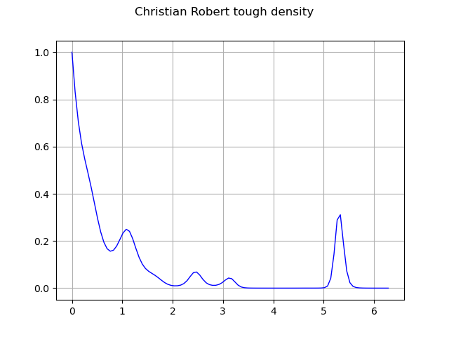
Draw the unnormalized probability density

import openturns as ot
from openturns.viewer import View
from numpy import pi
ot.RandomGenerator.SetSeed(1)
f = ot.SymbolicFunction(
    "x", "0.5 * (2 + sin(x)^2) * exp( -( 2 + cos(3*x)^3 + sin(2*x)^3) * x )")
lower_bound = 0.0
upper_bound = 2.0 * pi
graph = f.draw(lower_bound, upper_bound, 100)
graph.setTitle("Christian Robert tough density")
graph.setXTitle("")
graph.setYTitle("")
_ = View(graph)

Independent Metropolis-Hastings

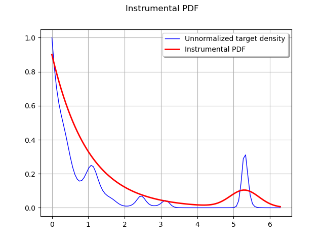
Let us use a mixture distribution to approximate the target distribution.

This approximation will serve as the instrumental distribution in the independent Metropolis-Hastings algorithm.

exp = ot.Exponential(1.0)
unif = ot.Normal(5.3, 0.4)
instrumentalDistribution = ot.Mixture([exp, unif], [0.9, 0.1])

Compare the instrumental density to the target density.

graph = f.draw(lower_bound, upper_bound, 100)
graph.setTitle("Instrumental PDF")
graph.setXTitle("")
graph.setYTitle("")
graph.add(instrumentalDistribution.drawPDF(lower_bound, upper_bound, 100))
graph.setLegendPosition("topright")
graph.setLegends(["Unnormalized target density", "Instrumental PDF"])
_ = View(graph)

MetropolisHastings and derived classes can work directly with the logarithm of the target density.

log_density = ot.ComposedFunction(ot.SymbolicFunction("x", "log(x)"), f)

In this case, it is easier to directly write it as a SymbolicFunction.

log_density = ot.SymbolicFunction(
    "x", "log(2 + sin(x)^2) - (2 + cos(3*x)^3 + sin(2*x)^3) * x")

initialState = ot.Point([3.0])  # not important in this case
support = ot.Interval([lower_bound], [upper_bound])
independentMH = ot.IndependentMetropolisHastings(
    log_density, support, initialState, instrumentalDistribution, [0])

Get a sample

sampleSize = 500
sample = independentMH.getSample(sampleSize)

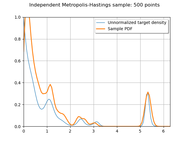
Plot the PDF of the sample to compare it to the target density

kernel = ot.KernelSmoothing()
posterior = kernel.build(sample)
graph = ot.Graph("Independent Metropolis-Hastings sample: {} points".format(
    sampleSize), "", "", True, "topright")
graph.setBoundingBox(ot.Interval(
    [lower_bound, 0.0], [upper_bound, f([0.0])[0]]))
graph.add(f.draw(lower_bound, upper_bound, 100))
graph.add(posterior.drawPDF(lower_bound, upper_bound, 100))
graph.setColors(ot.Drawable.BuildDefaultPalette(2))
graph.setLegends(["Unnormalized target density", "Sample PDF"])
_ = View(graph)

Even with very few sampling points (500), independent Metropolis-Hastings (with a judiciously chosen instrumental distribution) manages to capture the main features of the target density.

Random walk Metropolis-Hastings

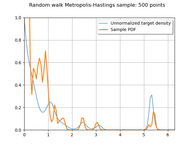
Let us use a normal instrumental distribution.

instrumentalDistribution = ot.Normal(0.0, 2.5)
randomwalkMH = ot.RandomWalkMetropolisHastings(
    log_density, support, initialState, instrumentalDistribution, [0])

Get a sample

sample = randomwalkMH.getSample(sampleSize)

Plot the PDF of the sample to compare it to the target density

kernel = ot.KernelSmoothing()
posterior = kernel.build(sample)
graph = ot.Graph("Random walk Metropolis-Hastings sample: {} points".format(
    sampleSize), "", "", True, "topright")
graph.setBoundingBox(ot.Interval(
    [lower_bound, 0.0], [upper_bound, f([0.0])[0]]))
graph.add(f.draw(lower_bound, upper_bound, 100))
graph.add(posterior.drawPDF(lower_bound, upper_bound, 100))
graph.setColors(ot.Drawable.BuildDefaultPalette(2))
graph.setLegends(["Unnormalized target density", "Sample PDF"])
_ = View(graph)

References

[1] Marin , J.M. & Robert, C.P. (2007). Bayesian Core: A Practical Approach to Computational Bayesian Statistics. Springer-Verlag, New York