Note
Click here to download the full example code
Create a spectral model
This use case illustrates how the User can define his own density spectral function from parametric models. The library allows it thanks to the object UserDefinedSpectralModel defined from:
a frequency grid
with step
, stored in the object RegularGrid,
a collection of hermitian matrices
stored in the object HermitianMatrixCollection, which are the images of each point of the frequency grid through the density spectral function.
The library builds a constant piecewise function on , where
the intervals where the density spectral function is constant are
centered on the points of the frequency grid, of length
.
Then, it is possible to evaluate the spectral density function for a
given frequency thanks to the method [computeSpectralDensity]{}: if
the frequency is not inside the interval
, an exception is thrown.
Otherwise, it returns the hermitian matrix of the
subinterval of
that contains the given frequency.
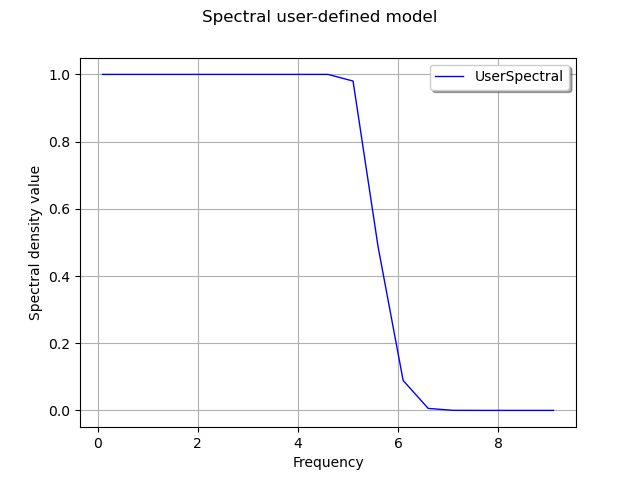
In the following script, we illustrate how to create a modified low
pass model of dimension with exponential decrease defined by:
where
Frequency value
should be positive,
for
, the spectral density function is constant:
,
for
, the spectral density function is equal to
.
The frequency grid is with
Hz.
The figure draws the spectral density.
import openturns as ot
import openturns.viewer as viewer
from matplotlib import pylab as plt
import math as m
ot.Log.Show(ot.Log.NONE)
Create the frequency grid:
fmin = 0.1
df = 0.5
N = int((10.0 - fmin) / df)
fgrid = ot.RegularGrid(fmin, df, N)
Define the spectral function:
def s(f):
    if(f <= 5.0):
        return 1.0
    else:
        x = f - 5.0
        return m.exp(-2.0 * x * x)
Create the collection of HermitianMatrix:
coll = ot.HermitianMatrixCollection()
for k in range(N):
    frequency = fgrid.getValue(k)
    matrix = ot.HermitianMatrix(1)
    matrix[0, 0] = s(frequency)
    coll.add(matrix)
Create the spectral model:
spectralModel = ot.UserDefinedSpectralModel(fgrid, coll)

# Get the spectral density function computed at first frequency values
firstFrequency = fgrid.getStart()
frequencyStep = fgrid.getStep()
firstHermitian = spectralModel(firstFrequency)

# Get the spectral function at frequency + 0.3 * frequencyStep
spectralModel(frequency + 0.3 * frequencyStep)
Draw the spectral density
# Create the curve of the spectral function
x = ot.Sample(N, 2)
for k in range(N):
    frequency = fgrid.getValue(k)
    x[k, 0] = frequency
    value = spectralModel(frequency)
    x[k, 1] = value[0, 0].real

# Create the graph
graph = ot.Graph('Spectral user-defined model', 'Frequency',
                 'Spectral density value', True)
curve = ot.Curve(x, 'UserSpectral')
graph.add(curve)
graph.setLegendPosition('topright')
view = viewer.View(graph)
plt.show()

Total running time of the script: ( 0 minutes 0.065 seconds)
 OpenTURNS