Note
Click here to download the full example code
Create a random walk process
This example details first how to create and manipulate a random walk.
A random walk is a process
where
discretized on the time grid
such
that:
where and
is a white noise of
dimension
.
The library proposes to model it through the object RandomWalk defined thanks to the origin, the distribution of the white noise and the time grid.
import openturns as ot
import openturns.viewer as viewer
from matplotlib import pylab as plt
import math as m
ot.Log.Show(ot.Log.NONE)
Define the origin
origin = [0.0]
Define an 1-d mesh
tgrid = ot.RegularGrid(0.0, 1.0, 500)
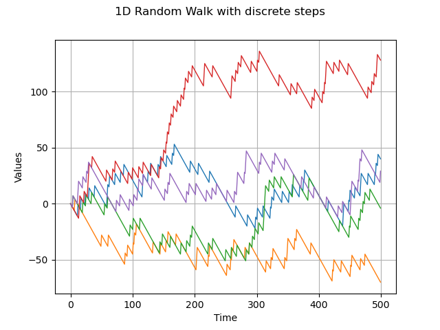
1-d random walk and discrete distribution
dist = ot.UserDefined([[-1], [10]], [0.9, 0.1])
process = ot.RandomWalk(origin, dist, tgrid)
sample = process.getSample(5)
graph = sample.drawMarginal(0)
graph.setTitle('1D Random Walk with discrete steps')
view = viewer.View(graph)

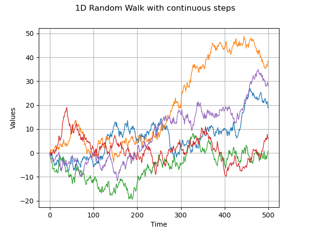
1-d random walk and continuous distribution
dist = ot.Normal(0.0, 1.0)
process = ot.RandomWalk(origin, dist, tgrid)
sample = process.getSample(5)
graph = sample.drawMarginal(0)
graph.setTitle('1D Random Walk with continuous steps')
view = viewer.View(graph)

Define the origin
origin = [0.0]*2
color palette
pal = ['red', 'cyan', 'blue', 'yellow', 'green']
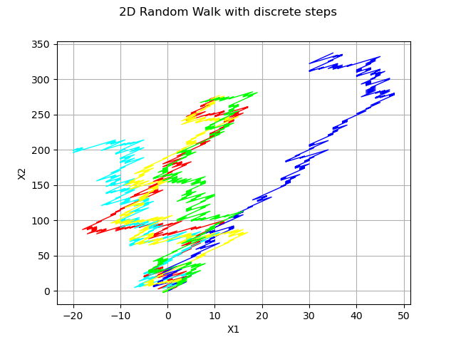
2-d random walk and discrete distribution
dist = ot.UserDefined([[-1., -2.], [1., 3.]], [0.5, 0.5])
process = ot.RandomWalk(origin, dist, tgrid)
sample = process.getSample(5)
graph = ot.Graph('2D Random Walk with discrete steps', 'X1', 'X2', True)
for i in range(5):
    graph.add(ot.Curve(sample[i], pal[i % len(pal)], 'solid'))
view = viewer.View(graph)

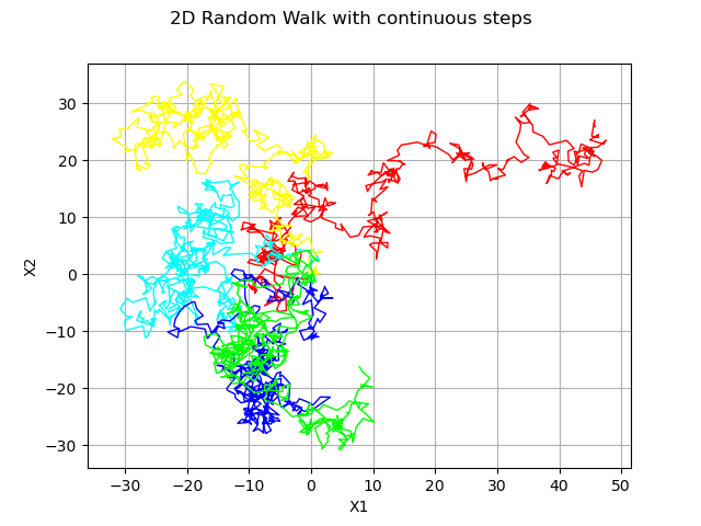
2-d random walk and continuous distribution
dist = ot.Normal(2)
process = ot.RandomWalk(origin, dist, tgrid)
sample = process.getSample(5)
graph = ot.Graph('2D Random Walk with continuous steps', 'X1', 'X2', True)
for i in range(5):
    graph.add(ot.Curve(sample[i], pal[i % len(pal)], 'solid'))
view = viewer.View(graph)
plt.show()

Total running time of the script: ( 0 minutes 0.321 seconds)
 OpenTURNS