Create a threshold event

Abstract

We present in this example the creation and the use of a ThresholdEvent to estimate a simple integral.

import openturns as ot
import openturns.viewer as otv
from matplotlib import pylab as plt

We consider a standard Gaussian random vector and build a random vector from this distribution.

distX = ot.Normal()
vecX = ot.RandomVector(distX)

We consider the simple model and consider the output random variable .

f = ot.SymbolicFunction(['x1'], ['abs(x1)'])
vecY = ot.CompositeRandomVector(f, vecX)

We define a very simple ThresholdEvent which happpens whenever :

thresholdEvent = ot.ThresholdEvent(vecY, ot.Less(), 1.0)

For the normal distribution, it is a well-known fact that the values lower than one standard deviation (here exactly 1) away from the mean (here 0) account roughly for 68.27% of the set. So the probability of the event is

print("Probability of the event : %.4f" % 0.6827)

Out:

Probability of the event : 0.6827

We can also use a basic estimator to get the probability of the event by drawing samples from the initial distribution distX and counting those which realize the event :

print("Probability of the event (event sampling) : %.4f" %
      thresholdEvent.getSample(1000).computeMean()[0])

Out:

Probability of the event (event sampling) : 0.6770

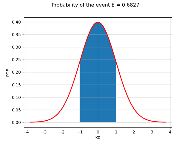
The geometric interpretation is simply the area under the PDF of the standard normal distribution for which we draw thereafter.

def linearSample(xmin, xmax, npoints):
    """
    Returns a sample created from a regular grid
    from xmin to xmax with npoints points.
    """
    step = (xmax-xmin)/(npoints-1)
    rg = ot.RegularGrid(xmin, step, npoints)
    vertices = rg.getVertices()
    return vertices

The boundary of the event are the lines and

a, b = -1, 1

nplot = 100  # Number of points in the plot
x = linearSample(a, b, nplot)
y = distX.computePDF(x)


def drawInTheBounds(vLow, vUp, n_test):
    """
    Draw the area within the bounds.
    """
    palette = ot.Drawable.BuildDefaultPalette(2)
    myPaletteColor = palette[0]
    polyData = [[vLow[i], vLow[i+1], vUp[i+1], vUp[i]]
                for i in range(n_test-1)]
    polygonList = [ot.Polygon(
        polyData[i], myPaletteColor, myPaletteColor) for i in range(n_test-1)]
    boundsPoly = ot.PolygonArray(polygonList)
    return boundsPoly


vLow = [[x[i, 0], 0.] for i in range(nplot)]
vUp = [[x[i, 0], y[i, 0]] for i in range(nplot)]
area = distX.computeCDF(b) - distX.computeCDF(a)
boundsPoly = drawInTheBounds(vLow, vUp, nplot)

We add the colored area to the PDF graph.

graph = distX.drawPDF()
graph.add(boundsPoly)
graph.setTitle("Probability of the event E = %.4f" % (area))
graph.setLegends([""])
view = otv.View(graph)

Display all figures

plt.show()