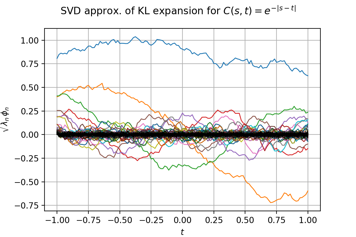
KarhunenLoeveSVDAlgorithm¶

(Source code, png, hires.png, pdf)

class KarhunenLoeveSVDAlgorithm(*args)¶

Computation of Karhunen-Loeve decomposition using SVD approximation.

Available constructors:

KarhunenLoeveSVDAlgorithm(sample, threshold, centeredSample)

KarhunenLoeveSVDAlgorithm(sample, verticesWeights, threshold, centeredSample)

KarhunenLoeveSVDAlgorithm(sample, verticesWeights, sampleWeights, threshold, centeredSample)

Parameters

sampleProcessSample: The sample containing the observations.
verticesWeightssequence of float: The weights associated to the vertices of the mesh defining the sample.
sampleWeightssequence of float: The weights associated to the fields of the sample.
thresholdpositive float, default=0.0: The threshold used to select the most significant eigenmodes, defined in KarhunenLoeveAlgorithm.
centeredSamplebool, default=False: Flag to tell if the sample is drawn according to a centered process or if it has to be centered using the empirical mean.

Notes

The Karhunen-Loeve SVD algorithm solves the Fredholm problem associated to the covariance function $C$ : see KarhunenLoeveAlgorithm to get the notations.

The SVD approach is a particular case of the quadrature approach (see KarhunenLoeveQuadratureAlgorithm) where we consider the functional basis $((\vect{\theta}_p^j(\vect{s}))_{1 \leq j \leq d, 1 \leq p \leq P}$ of $L^2(\cD, \Rset^d)$ defined on $\cD$ by:

$\vect{\theta}_p^j(\vect{s})= \left[\mat{C}(\vect{s}, \vect{s}_p) \right]_{:, j}$

The SVD approach is used when the covariance function is not explicitly known but only through $K$ fields of the associated stochastic process $\vect{X}$ : $(\vect{X}_1, \dots, \vect{X}_K)$ .

It consists in :

approximating $\mat{C}$ by its empirical estimator $\dfrac{1}{\tilde{K}} \tilde{\mat{X}}\, \Tr{\tilde{\mat{X}}}$ where $\tilde{\mat{X}}~=~(\vect{X}_1 | \dots | \vect{X}_K)$ and $\tilde{K}=K$ if the process is centered and $\tilde{\mat{X}}~=~(\vect{X}_1 - \vect{\mu} | \dots | \vect{X}_K - \vect{\mu})$ $\tilde{K}=K-1$ otherwise, where $\vect{\mu}=\dfrac{1}{K}\sum_{k=1}^K\vect{X}_k$ ;

taking the $L$ vertices of the mesh of $\vect{X}$ as the $L$ quadrature points.

We suppose now that $K < dL$ , and we note $\mat{Y} = \sqrt{\mat{W}} \,\mat{X}$ .

As the matrix $\mat{\Theta} = \mat{C}$ is invertible, the Galerkin and collocation approaches are equivalent and both lead to the following singular value problem for $\mat{Y}$ :

(1)¶ $\mat{Y}\,\Tr{\mat{Y}}\,\mat{\Psi}_k & = \tilde{K} \lambda_k \mat{\Psi}_k$

The SVD decomposition of $\mat{Y}\in \mathcal{M}_{dL,\tilde{K}}(\Rset)$ writes:

$\mat{Y} = \mat{U}\, \mat{\Sigma} \, \Tr{\mat{V}}$

where we have $\mat{U} \in \mathcal{M}_{dL,\tilde{K}}(\Rset)$ , $\mat{\Sigma}\in \mathcal{M}_{\tilde{K},\tilde{K}}(\Rset)$ , $\mat{V} \in \mathcal{M}_{\tilde{K},\tilde{K}}(\Rset)$ such that :

$\Tr{\mat{V}}\mat{V} =\mat{V}\Tr{\mat{V}}= \mat{I}_{\tilde{K}}$ ,

$\Tr{\mat{U}}\mat{U} = \mat{I}_{\tilde{K}}$ ,

$\mat{\Sigma} = diag(\sigma_1, \dots, \sigma_{\tilde{K}})$ .

Then the columns of $\mat{U}$ are the eigenvectors of $\mat{Y}\Tr{\mat{Y}}$ associated to the eigenvalues $\sigma_k^2$ .

We deduce the modes and eigenvalues of the Fredholm problem for $k \leq \tilde{K}$ :

$\begin{align*} \mat{\Phi}_k = \dfrac{1}{\lambda_k} \sqrt{\mat{W}}\, \mat{U}_k \lambda_k = \dfrac{\sigma_k^2}{\tilde{K}} \end{align*}$

We have:

$\tilde{\vect{\varphi}}_k(\vect{t})= \sum_{\ell=1}^L C(\vect{t}, \vect{\xi}_\ell) \vect{\phi}_{\ell,k} \quad \mbox{pour} \quad k \leq \tilde{K}$

The most computationally intensive part of the algorithm is the computation of the SVD decomposition. By default, it is done using LAPACK dgesdd routine. While being very accurate and reasonably fast for small to medium sized problems, it becomes prohibitively slow for large cases. The user can choose to use a stochastic algorithm instead, with the constraint that the number of singular values to be computed has to be fixed a priori. The following keys of ResourceMap allow to select and tune these algorithms:

‘KarhunenLoeveSVDAlgorithm-UseRandomSVD’ which triggers the use of a random algorithm. By default, it is set to False and LAPACK is used.

‘KarhunenLoeveSVDAlgorithm-RandomSVDMaximumRank’ which fixes the number of singular values to compute. By default it is set to 1000.

‘KarhunenLoeveSVDAlgorithm-RandomSVDVariant’ which can be equal to either ‘halko2010’ for [halko2010] (the default) or ‘halko2011’ for [halko2011]. These two algorithms have very similar structures, the first one being based on a random compression of both the rows and columns of $\mat{Y}$ , the second one being based on an iterative compressed sampling of the columns of $\mat{Y}$ .

‘KarhunenLoeveSVDAlgorithm-halko2011Margin’ and ‘KarhunenLoeveSVDAlgorithm-halko2011Iterations’ to fix the parameters of the ‘halko2011’ variant. See [halko2011] for the details.

Examples

Create a Karhunen-Loeve SVD algorithm:

>>> import openturns as ot
>>> mesh = ot.IntervalMesher([10]*2).build(ot.Interval([-1.0]*2, [1.0]*2))
>>> s = 0.01
>>> model = ot.AbsoluteExponential([1.0]*2)
>>> sample = ot.GaussianProcess(model, mesh).getSample(8)
>>> algorithm = ot.KarhunenLoeveSVDAlgorithm(sample, s)

Run it!

>>> algorithm.run()
>>> result = algorithm.getResult()

Methods

`getClassName`()	Accessor to the object's name.
`getCovarianceModel`()	Accessor to the covariance model.
`getId`()	Accessor to the object's id.
`getName`()	Accessor to the object's name.
`getNbModes`()	Accessor to number of modes to compute.
`getResult`()	Get the result structure.
`getSample`()	Accessor to the process sample.
`getSampleWeights`()	Accessor to the weights of the sample.
`getShadowedId`()	Accessor to the object's shadowed id.
`getThreshold`()	Accessor to the threshold used to select the most significant eigenmodes.
`getVerticesWeights`()	Accessor to the weights of the vertices.
`getVisibility`()	Accessor to the object's visibility state.
`hasName`()	Test if the object is named.
`hasVisibleName`()	Test if the object has a distinguishable name.
`run`()	Computation of the eigenvalues and eigenfunctions values at nodes.
`setCovarianceModel`(covariance)	Accessor to the covariance model.
`setName`(name)	Accessor to the object's name.
`setNbModes`(nbModes)	Accessor to the maximum number of modes to compute.
`setShadowedId`(id)	Accessor to the object's shadowed id.
`setThreshold`(threshold)	Accessor to the limit ratio on eigenvalues.
`setVisibility`(visible)	Accessor to the object's visibility state.

__init__(*args)¶

getClassName()¶

Accessor to the object’s name.

Returns

class_namestr: The object class name (object.__class__.__name__).

getCovarianceModel()¶

Accessor to the covariance model.

Returns

covModelCovarianceModel: The covariance model.

getId()¶

Accessor to the object’s id.

Returns

idint: Internal unique identifier.

getName()¶

Accessor to the object’s name.

Returns

namestr: The name of the object.

getNbModes()¶

Accessor to number of modes to compute.

Returns

nint: The maximum number of modes to compute. The actual number of modes also depends on the threshold criterion.

getResult()¶

Get the result structure.

Returns

resKLKarhunenLoeveResult: The structure containing all the results of the Fredholm problem.

Notes

The structure contains all the results of the Fredholm problem.

getSample()¶

Accessor to the process sample.

Returns

sampleProcessSample: The process sample containing the observations of the process.

getSampleWeights()¶

Accessor to the weights of the sample.

Returns

weightsPoint: The weights associated to the fields of the sample.

Notes

The fields might not have the same weight, for example if they come from importance sampling.

getShadowedId()¶

Accessor to the object’s shadowed id.

Returns

idint: Internal unique identifier.

getThreshold()¶

Accessor to the threshold used to select the most significant eigenmodes.

Returns

sfloat, positive: The threshold $s$ .

Notes

OpenTURNS truncates the sequence $(\lambda_k, \vect{\varphi}_k)_{k \geq 1}$ at the index $K$ defined in (3).

getVerticesWeights()¶

Accessor to the weights of the vertices.

Returns

weightsPoint: The weights associated to the vertices of the mesh defining the sample field.

Notes

The vertices might not have the same weight, for example if the mesh is not regular.

getVisibility()¶

Accessor to the object’s visibility state.

Returns

visiblebool: Visibility flag.

hasName()¶

Test if the object is named.

Returns

hasNamebool: True if the name is not empty.

hasVisibleName()¶

Test if the object has a distinguishable name.

Returns

hasVisibleNamebool: True if the name is not empty and not the default one.

run()¶

Computation of the eigenvalues and eigenfunctions values at nodes.

Notes

Runs the algorithm and creates the result structure KarhunenLoeveResult.

setCovarianceModel(covariance)¶

Accessor to the covariance model.

Parameters

covModelCovarianceModel: The covariance model.

setName(name)¶

Accessor to the object’s name.

Parameters

namestr: The name of the object.

setNbModes(nbModes)¶

Accessor to the maximum number of modes to compute.

Parameters

nint: The maximum number of modes to compute. The actual number of modes also depends on the threshold criterion.

setShadowedId(id)¶

Accessor to the object’s shadowed id.

Parameters

idint: Internal unique identifier.

setThreshold(threshold)¶

Accessor to the limit ratio on eigenvalues.

Parameters

sfloat, $\geq 0$: The threshold $s$ defined in (3).

setVisibility(visible)¶

Accessor to the object’s visibility state.

Parameters

visiblebool: Visibility flag.

OpenTURNS

An Open source initiative for the Treatment of Uncertainties, Risks'N Statistics

Previous topic

Next topic

This Page

KarhunenLoeveSVDAlgorithm¶