TaylorExpansionMoments¶

class TaylorExpansionMoments(*args)¶

First and second order Taylor expansion formulas.

Refer to Taylor decomposition importance factors.

Parameters:

limitStateVariableRandomVector: It must be of type Composite, which means it must have been defined with the class CompositeRandomVector.

Notes

Assuming that $\uX$ has its two first moments finite and that $h$ is sufficiently regular, the Taylor expansion method is used to approximate the mean and variance of a random variable $\uY = h(\uX)$ with respect to the mean and variance of the input random vector $\uX$ .

We note:

$\mu_X = \Expect{\uX}$ the mean of the random vector $\uX$
$\Cov \uX$ the covariance matrix of the random vector $\uX$ . The elements are the followings : $(\Cov \uX)_{ij} = \Expect{\left(X^i - \Expect{X^i} \right) \left(X^j - \Expect{X^j} \right) }$
$\vect{\vect{\nabla}} h(\muX) = \: \Tr{\left( \frac{\partial y^i}{\partial x^j}\right)}_{\ux\: =\: \muX} = \: \Tr{\left( \frac{\partial h^i(\ux)}{\partial x^j}\right)}_{\ux\: =\: \muX}$ is the transposed Jacobian matrix with $i=1,\ldots,n_Y$ and $j=1,\ldots,n_X$ .
$\vect{\vect{\vect{\nabla^2}}} h(\ux\:,\ux)$ is a tensor of order 3. It is composed by the second order derivative towards the $i^\textrm{th}$ and $j^\textrm{th}$ components of $\ux$ of the $k^\textrm{th}$ component of the output vector $h(\ux)$ . It yields to: $\left( \nabla^2 h(\ux) \right)_{ijk} = \frac{\partial^2 (h^k(\ux))}{\partial x^i \partial x^j}$

Then we have:

$<\vect{\vect{\nabla}}h(\muX) , \: \uX - \muX> = \sum_{j=1}^{n_X} \left( \frac{\partial {\uy}}{\partial {x^j}}\right)_{\ux = \muX} . \left( X^j-\muX^j \right)$

and

$<<\vect{\vect{\vect{\nabla }}}^2 h(\muX,\: \vect{\mu}_{X}),\: \uX - \muX>,\: \uX - \muX> = \left( \Tr{(\uX^i - \muX^i)}. \left(\frac{\partial^2 y^k}{\partial x^i \partial x^k}\right)_{\ux = \muX}. (\uX^j - \muX^j) \right)_{ijk}$

The Taylor expansion of order 2 of the model $h$ is:

$\uY = h(\muX) + <\vect{\vect{\nabla}}h(\muX) , \: \uX - \muX> + \frac{1}{2}<<\vect{\vect{\vect{\nabla }}}^2 h(\muX,\: \vect{\mu}_{\:X}),\: \uX - \muX>,\: \uX - \muX> + o(\Cov \uX)$

Depending on the order of the Taylor expansion (classically first order or second order), one can obtain different formulas introduced hereafter.

Approximation at the order 1:

Expectation:

$\Expect{\uY} \approx \vect{h}(\muX)$

Pay attention that $\Expect{\uY}$ is a vector. The $k^\textrm{th}$ component of this vector is equal to the $k^\textrm{th}$ component of the output vector computed by the model $h$ at the mean value. $\Expect{\uY}$ is thus the computation of the model at mean.

Variance:

$\Cov \uY \approx \Tr{\vect{\vect{\nabla}}}\:\vect{h}(\muX).\Cov \uX.\vect{\vect{\nabla}}\:\vect{h}(\muX)$

Approximation at the order 2:

Expectation:

$(\Expect{\uY})_k \approx (\vect{h}(\muX))_k + \left( \sum_{i=1}^{n_X}\frac{1}{2} (\Cov \uX)_{ii}.{(\nabla^2\:h(\uX))}_{iik} + \sum_{i=1}^{n_X} \sum_{j=1}^{i-1} (\Cov X)_{ij}.{(\nabla^2\:h(\uX))}_{ijk} \right)_k$

Variance:

The decomposition of the variance at the order 2 is not implemented. It requires both the knowledge of higher order derivatives of the model and the knowledge of moments of order strictly greater than 2 of the PDF.

Examples

>>> import openturns as ot
>>> ot.RandomGenerator.SetSeed(0)
>>> myFunc = ot.SymbolicFunction(['x1', 'x2', 'x3', 'x4'],
...     ['(x1*x1+x2^3*x1)/(2*x3*x3+x4^4+1)', 'cos(x2*x2+x4)/(x1*x1+1+x3^4)'])
>>> R = ot.CorrelationMatrix(4)
>>> for i in range(4):
...     R[i, i - 1] = 0.25
>>> distribution = ot.Normal([0.2]*4, [0.1, 0.2, 0.3, 0.4], R)
>>> # We create a distribution-based RandomVector
>>> X = ot.RandomVector(distribution)
>>> # We create a composite RandomVector Y from X and myFunc
>>> Y = ot.CompositeRandomVector(myFunc, X)
>>> # We create a Taylor expansion method to approximate moments
>>> myTaylorExpansionMoments = ot.TaylorExpansionMoments(Y)
>>> print(myTaylorExpansionMoments.getMeanFirstOrder())
[0.0384615,0.932544]

Methods

`drawImportanceFactors`()	Draw the importance factors.
`getClassName`()	Accessor to the object's name.
`getCovariance`()	Get the approximation at the first order of the covariance matrix.
`getGradientAtMean`()	Get the gradient of the function.
`getHessianAtMean`()	Get the hessian of the function.
`getId`()	Accessor to the object's id.
`getImportanceFactors`()	Get the importance factors.
`getLimitStateVariable`()	Get the limit state variable.
`getMeanFirstOrder`()	Get the approximation at the first order of the mean.
`getMeanSecondOrder`()	Get the approximation at the second order of the mean.
`getName`()	Accessor to the object's name.
`getShadowedId`()	Accessor to the object's shadowed id.
`getValueAtMean`()	Get the value of the function.
`getVisibility`()	Accessor to the object's visibility state.
`hasName`()	Test if the object is named.
`hasVisibleName`()	Test if the object has a distinguishable name.
`setName`(name)	Accessor to the object's name.
`setShadowedId`(id)	Accessor to the object's shadowed id.
`setVisibility`(visible)	Accessor to the object's visibility state.

__init__(*args)¶

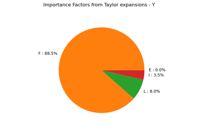
drawImportanceFactors()¶

Draw the importance factors.

Returns:

graphGraph: Graph containing the pie corresponding to the importance factors of the probabilistic variables.

getClassName()¶

Accessor to the object’s name.

Returns:

class_namestr: The object class name (object.__class__.__name__).

getCovariance()¶

Get the approximation at the first order of the covariance matrix.

Returns:

covarianceCovarianceMatrix: Approximation at the first order of the covariance matrix of the random vector.

getGradientAtMean()¶

Get the gradient of the function.

Returns:

gradientMatrix: Gradient of the Function which defines the random vector at the mean point of the input random vector.

getHessianAtMean()¶

Get the hessian of the function.

Returns:

hessianSymmetricTensor: Hessian of the Function which defines the random vector at the mean point of the input random vector.

getId()¶

Accessor to the object’s id.

Returns:

idint: Internal unique identifier.

getImportanceFactors()¶

Get the importance factors.

Returns:

factorsPoint: Importance factors of the inputs : only when randVect is of dimension 1.

getLimitStateVariable()¶

Get the limit state variable.

Returns:

limitStateVariableRandomVector: Limit state variable.

getMeanFirstOrder()¶

Get the approximation at the first order of the mean.

Returns:

meanPoint: Approximation at the first order of the mean of the random vector.

getMeanSecondOrder()¶

Get the approximation at the second order of the mean.

Returns:

meanPoint: Approximation at the second order of the mean of the random vector (it requires that the hessian of the Function has been defined).

getName()¶

Accessor to the object’s name.

Returns:

namestr: The name of the object.

getShadowedId()¶

Accessor to the object’s shadowed id.

Returns:

idint: Internal unique identifier.

getValueAtMean()¶

Get the value of the function.

Returns:

valuePoint: Value of the Function which defines the random vector at the mean point of the input random vector.

getVisibility()¶

Accessor to the object’s visibility state.

Returns:

visiblebool: Visibility flag.

hasName()¶

Test if the object is named.

Returns:

hasNamebool: True if the name is not empty.

hasVisibleName()¶

Test if the object has a distinguishable name.

Returns:

hasVisibleNamebool: True if the name is not empty and not the default one.

setName(name)¶

Accessor to the object’s name.

Parameters:

namestr: The name of the object.

setShadowedId(id)¶

Accessor to the object’s shadowed id.

Parameters:

idint: Internal unique identifier.

setVisibility(visible)¶

Accessor to the object’s visibility state.

Parameters:

visiblebool: Visibility flag.

Examples using the class¶

Analyse the central tendency of a cantilever beam

Estimate moments from Taylor expansions

Example of sensitivity analyses on the wing weight model

OpenTURNS

An Open source initiative for the Treatment of Uncertainties, Risks'N Statistics

Table of Contents

Previous topic

Next topic

This Page

TaylorExpansionMoments¶

Examples using the class¶