GeneralizedExtremeValueFactory¶

(Source code, png)

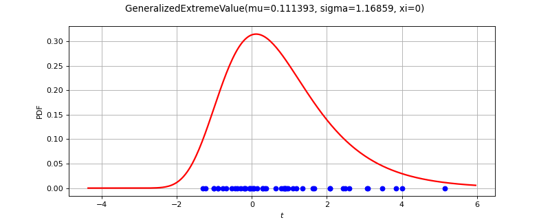
class GeneralizedExtremeValueFactory(*args)¶

GeneralizedExtremeValue factory.

See also

DistributionFactory, GeneralizedExtremeValue, FrechetFactory, GumbelFactory, WeibullMaxFactory

Methods

`build`(*args)	Estimate the distribution as a `Frechet`, `Gumbel` or `WeibullMax` distribution.
`buildAsGeneralizedExtremeValue`(*args)	Estimate the distribution as a `Frechet`, `Gumbel` or `WeibullMax` distribution.
`buildEstimator`(*args)	Build the distribution and the parameter distribution.
`buildMethodOfLikelihoodMaximization`(sample)	Estimate the distribution from the $r$ largest order statistics.
`buildMethodOfLikelihoodMaximizationEstimator`(sample)	Estimate the distribution and the parameter distribution with the R-maxima method.
`buildMethodOfProfileLikelihoodMaximization`(sample)	Estimate the distribution with the profile likelihood.
`buildMethodOfProfileLikelihoodMaximizationEstimator`(sample)	Estimate the distribution and the parameter distribution with the profile likelihood.
`buildReturnLevelEstimator`(result, m)	Estimate a return level and its distribution from the GEV parameters.
`buildReturnLevelProfileLikelihood`(sample, m)	Estimate a return level and its distribution with the profile likelihood.
`buildReturnLevelProfileLikelihoodEstimator`(...)	Estimate $(z_m, \sigma, \xi)$ and its distribution with the profile likelihood.
`buildTimeVarying`(*args)	Estimate a non stationary GEV.
`getBootstrapSize`()	Accessor to the bootstrap size.
`getClassName`()	Accessor to the object's name.
`getId`()	Accessor to the object's id.
`getName`()	Accessor to the object's name.
`getShadowedId`()	Accessor to the object's shadowed id.
`getVisibility`()	Accessor to the object's visibility state.
`hasName`()	Test if the object is named.
`hasVisibleName`()	Test if the object has a distinguishable name.
`setBootstrapSize`(bootstrapSize)	Accessor to the bootstrap size.
`setName`(name)	Accessor to the object's name.
`setShadowedId`(id)	Accessor to the object's shadowed id.
`setVisibility`(visible)	Accessor to the object's visibility state.

__init__(*args)¶

build(*args)¶

Estimate the distribution as a Frechet, Gumbel or WeibullMax distribution.

Available usages:

build(sample)

build(param)

Parameters:

sample2-d sequence of float: The block maxima sample of dimension 1.
paramCollection of PointWithDescription: A vector of parameters of the distribution.

Returns:

distributionGeneralizedExtremeValue: The estimated distribution.

Notes

The strategy consists in fitting the three models Frechet, Gumbel and WeibullMax on the data. Then, the three models are classified with respect to the BIC criterion. The best one is returned.

buildAsGeneralizedExtremeValue(*args)¶

Estimate the distribution as a Frechet, Gumbel or WeibullMax distribution.

Same as build().

buildEstimator(*args)¶

Build the distribution and the parameter distribution.

Parameters:

sample2-d sequence of float: Sample from which the distribution parameters are estimated.
parametersDistributionParameters: Optional, the parametrization.

Returns:

resDistDistributionFactoryResult: The results.

Notes

According to the way the native parameters of the distribution are estimated, the parameters distribution differs:

Moments method: the asymptotic parameters distribution is normal and estimated by Bootstrap on the initial data;

Maximum likelihood method with a regular model: the asymptotic parameters distribution is normal and its covariance matrix is the inverse Fisher information matrix;

Other methods: the asymptotic parameters distribution is estimated by Bootstrap on the initial data and kernel fitting (see KernelSmoothing).

If another set of parameters is specified, the native parameters distribution is first estimated and the new distribution is determined from it:

if the native parameters distribution is normal and the transformation regular at the estimated parameters values: the asymptotic parameters distribution is normal and its covariance matrix determined from the inverse Fisher information matrix of the native parameters and the transformation;

in the other cases, the asymptotic parameters distribution is estimated by Bootstrap on the initial data and kernel fitting.

buildMethodOfLikelihoodMaximization(sample, r=0)¶

Estimate the distribution from the $r$ largest order statistics.

Let us suppose we have a series of independent and identically distributed variables and that data are grouped into $n$ blocks. In each block, the largest $R$ observations are recorded.

We define the series $M_i^{(R)} = (z_i^{(1)}, \hdots, z_i^{(R)})$ for $1 \leq i \leq n$ where the values are sorted in decreasing order.

The estimator of $(\mu, \sigma, \xi)$ maximizes the log-likelihood built from the $r$ largest order statisctics, with $1 \leq r \leq R$ defined as:

If $\xi \neq 0$ , then:

(1)¶ $\ell(\mu, \sigma, \xi) = -nr \log \sigma - \sum_{i=1}^n \biggl[ 1 + \xi \Bigl( \frac{z_i^{(r)} - \mu }{\sigma} \Bigr) \biggr]^{-1/\xi} -\left(\dfrac{1}{\xi} +1 \right) \sum_{i=1}^n \sum_{k=1}^r \log \biggl[ 1 + \xi \Bigl( \frac{z_i^{(k)} - \mu }{\sigma} \Bigr) \biggr]$

defined on $(\mu, \sigma, \xi)$ such that $1+\xi \left( \frac{z_i^{(k)} - \mu}{\sigma} \right) > 0$ for all $1 \leq i \leq m$ and $1 \leq k \leq r$ .

If $\xi = 0$ , then:

(2)¶ $\ell(\mu, \sigma, \xi) = -nr \log \sigma - \sum_{i=1}^n \exp \biggl[ - \Bigl( \frac{z_i^{(r)} - \mu }{\sigma} \Bigr) \biggr] - \sum_{i=1}^n \sum_{k=1}^r \Bigl( \frac{z_i^{(k)} - \mu }{\sigma} \Bigr)$

Parameters:

sample2-d sequence of float

Block maxima grouped in a sample of size $n$ and dimension $R$ .

rint, $1 \leq r \leq R$ ,

Number of largest order statistics taken into account among the $R$ stored ones.

By default, $r=0$ which means that all the maxima are used.

Returns:

distributionGeneralizedExtremeValue: The estimated distribution.

buildMethodOfLikelihoodMaximizationEstimator(sample, r=0)¶

Estimate the distribution and the parameter distribution with the R-maxima method.

The estimators are defined using the profile log-likelihood as detailed in buildMethodOfLikelihoodMaximization().

The result class produced by the method provides:

the GEV distribution associated to $(\hat{\mu}, \hat{\sigma}, \hat{\xi})$ ,
the asymptotic distribution of $(\hat{\mu}, \hat{\sigma}, \hat{\xi})$ .

Parameters:

sampleM2-d sequence of float

Block maxima grouped in a sample of size $n$ and dimension $R$ .

rint, $1 \leq r \leq R$ , optional

Number of order statistics taken into account among the $R$ stored ones.

By default, $r=0$ which means that all the maxima are used.

Returns:

resultDistributionFactoryLikelihoodResult: The result class.

buildMethodOfProfileLikelihoodMaximization(sample)¶

Estimate the distribution with the profile likelihood.

The estimator $(\hat{\mu}, \hat{\sigma}, \hat{\xi})$ is defined using a nested numerical optimization of the log-likelihood:

$\ell_p (\xi) = \max_{(\mu, \sigma)} \ell (\mu, \sigma, \xi)$

where $\ell (\mu, \sigma, \xi)$ is detailed in equations (1) and (2) with $r=1$ .

The estimator is given by:

$\begin{align*} \hat{\xi} & = \argmax_{\xi} \ell_p(\xi)\\ (\hat{\mu}, \hat{\sigma}) & = \argmax_{(\mu, \sigma)} \ell(\mu, \sigma, \hat{\xi}) \end{align*}$

Parameters:

sample2-d sequence of float: The block maxima sample of dimension 1.

Returns:

distributionGeneralizedExtremeValue: The estimated distribution.

Notes

The starting point of the optimization is initialized from the probability weighted moments method, see [diebolt2008].

buildMethodOfProfileLikelihoodMaximizationEstimator(sample)¶

Estimate the distribution and the parameter distribution with the profile likelihood.

The estimators are defined in buildMethodOfProfileLikelihoodMaximization().

The result class produced by the method provides:

the GEV distribution associated to $(\hat{\mu}, \hat{\sigma}, \hat{\xi})$ ,
the asymptotic distribution of $(\hat{\mu}, \hat{\sigma}, \hat{\xi})$ ,
the profile log-likelihood function $\xi \mapsto \ell_p(\xi)$ ,
the optimal profile log-likelihood value $\ell_p(\hat{\xi})$ ,
confidence intervals of level $(1-\alpha)$ of $\xi$ .

Parameters:

sample2-d sequence of float: The block maxima sample of dimension 1.

Returns:

resultProfileLikelihoodResult: The result class.

buildReturnLevelEstimator(result, m)¶

Estimate a return level and its distribution from the GEV parameters.

The $m$ -return level $z_m$ is the level exceeded on average once every $m$ blocks. The parameter $m$ is referred to as the return period. For example, if the GEV distribution is the distribution of the annual maxima, then $z_{100}$ is the 100-year return period and is exceeded on average once in every century.

The $m$ -return level is defined as the quantile of order $1-p=1-1/m$ of the GEV distribution.

If $\xi \neq 0$ :

(3)¶ $z_m = \mu - \frac{\sigma}{\xi} \left[ 1- (-\log(1-p))^{-\xi}\right]$

If $\xi = 0$ :

(4)¶ $z_m = \mu - \sigma \log(-\log(1-p))$

The estimator $\hat{z}_m$ of $z_m$ is deduced from the estimator $(\hat{\mu}, \hat{\sigma}, \hat{\xi})$ of $(\mu, \sigma, \xi)$ .

The asymptotic distribution of $\hat{z_m}$ is obtained by the Delta method from the asymptotic distribution of $(\hat{\mu}, \hat{\sigma}, \hat{\xi})$ . It is a normal distribution with mean $\hat{z}_m$ and variance:

$\Var{z_m} = (\nabla z_m)^T \mat{V}_n \nabla z_m$

where $\nabla z_m = (\frac{\partial z_m}{\partial \mu}, \frac{\partial z_m}{\partial \sigma}, \frac{\partial z_m}{\partial \xi})$ and $\mat{V}_n$ is the asymptotic covariance of $(\hat{\mu}, \hat{\sigma}, \hat{\xi})$ .

Parameters:

resultDistributionFactoryResult: Likelihood estimation result of a GeneralizedExtremeValue
mfloat: The return period expressed in terms of number of blocks.

Returns:

distributionDistribution: The asymptotic distribution of $\hat{z}_m$ .

buildReturnLevelProfileLikelihood(sample, m)¶

Estimate a return level and its distribution with the profile likelihood.

The estimator is defined using a nested numerical optimization of the log-likelihood:

$\ell_p (z_m) = \max_{(\mu, \sigma)} \ell (z_m, \sigma, \xi)$

where $\ell (z_m, \sigma, \xi)$ is the log-likelihood detailed in (1) and (2) with $r=1$ and where we substitued $\mu$ for $z_m$ using equations (3) or (4).

The estimator $\hat{z}_m$ of $z_m$ is defined by:

$\hat{z}_m = \argmax_{z_m} \ell_p(z_m)$

The asymptotic distribution of $\hat{z}_m$ is normal.

Parameters:

sample2-d sequence of float: The block maxima sample of dimension 1.

Returns:

distributionNormal: The asymptotic distribution of $\hat{z}_m$ .

Notes

The starting point of the optimization is initialized from the regular maximum likelihood method.

buildReturnLevelProfileLikelihoodEstimator(sample, m)¶

Estimate $(z_m, \sigma, \xi)$ and its distribution with the profile likelihood.

The estimators are defined in buildReturnLevelProfileLikelihood().

The parameter estimates are given by:

$\begin{align*} \hat{z}_m = \argmax_{z_m} \ell_p(z_m)\\ (\hat{\sigma}, \hat{\xi}) = \argmax_{(\sigma, \xi)} \ell(\hat{z}_m, \sigma, \xi) \end{align*}$

The result class produced by the method provides:

the GEV distribution associated to $(\hat{z}_m, \hat{\sigma}, \hat{\xi})$ ,
the asymptotic distribution of $(\hat{z}_m, \hat{\sigma}, \hat{\xi})$ ,
the profile log-likelihood function $z_m \mapsto \ell_p(z_m)$ ,
the optimal profile log-likelihood value $\ell_p(\hat{z}_m)$ ,
confidence intervals of level $(1-\alpha)$ of $\hat{z}_m$ .

Parameters:

sample2-d sequence of float: The block maxima sample of dimension 1.
mfloat: The return period, defines the level of the quantile as $1-1/m$ .

Returns:

resultProfileLikelihoodResult: The result class.

buildTimeVarying(*args)¶

Estimate a non stationary GEV.

We consider a non stationary GEV model to describe the distribution of $Z_t$ :

$Z_t \sim \mbox{GEV}(\mu(t), \sigma(t), \xi(t))$

We have the values of $Z_t$ on the time stamps $(t_1, \dots, t_n)$ .

For numerical reasons, it is recommended to normalize the time stamps. OpenTURNS applies the following mapping:

$\tau(t) = \dfrac{t-c}{d}$

and with three ways of defining $(c,d)$ :

the CenterReduce method where $c = \dfrac{1}{n} \sum_{i=1}^n t_i$ is the mean time stamps and $d = \sqrt{\dfrac{1}{n} \sum_{i=1}^n (t_i-c)^2}$ is the standard deviation of the time stamps;
the MinMax method where $c = t_1$ is the first time and $d = t_n-t_1$ the range of the time stamps;
the None method where $c = 0$ and $d = 1$ : in that case, data are not normalized.

Each of $\mu(t), \sigma(t), \xi(t)$ has an expression in terms of a parameter vector and time functions:

$\theta(t) = h\left(\sum_{i=1}^{d_{\theta}} \beta_i^{\theta} \varphi_i^{\theta}(\tau(t))\right)$

where:

$h: \Rset \mapsto \Rset$ is usually referred to as the inverse-link function. The function $\theta(t)$ denotes either $\mu(t)$ , $\sigma(t)$ or $\xi(t)$ ,
each $\varphi_i^{\theta}$ is a scalar function $\Rset \mapsto \Rset$ ,
each $\beta_i^{j} \in \Rset$ .

We denote by $d_{\mu}$ , $d_{\sigma}$ and $d_{\xi}$ the size of the functional basis of $\mu$ , $\sigma$ and $\xi$ respectively. We denote by $\vect{\beta} = (\beta_1^{\mu}, \dots, \beta_{d_{\mu}}^{\mu}, \beta_1^{\sigma}, \dots, \beta_{d_{\sigma}}^{\sigma}, \beta_1^{\xi}, \dots, \beta_{d_{\xi}}^{\xi})$ the complete vector of parameters.

The estimator of $\vect{\beta}$ maximizes the likelihood of the non stationary model which is defined by:

$L(\vect{\beta}) = \prod_{t=1}^{n} g(z_{t};\mu(t), \sigma(t), \xi(t))$

where $g(z_{t};\mu(t), \sigma(t), \xi(t))$ denotes the GEV density function with parameters $\mu(t), \sigma(t), \xi(t)$ evaluated at $z_t$ .

Then, if none of the $\xi(t)$ is zero, the log-likelihood is defined by:

$\ell (\vect{\beta}) = -\sum_{t=1}^{n} \left\{ \log(\sigma(t)) + (1 + 1 / \xi(t) ) \log\left[ 1+\xi(t) \left( \frac{z_t - \mu(t)}{\sigma(t)}\right) \right] + \left[ 1 + \xi(t) \left( \frac{z_t- \mu(t)}{\sigma(t)} \right) \right]^{-1 / \xi(t)} \right\}$

defined on $(\mu, \sigma, \xi)$ such that $1+\xi \left( \frac{z_t - \mu}{\sigma} \right) > 0$ for all $t$ .

And if any of the $\xi(t)$ is equal to 0, the log-likelihood is defined as:

$\ell (\vect{\beta}) = -\sum_{t=1}^{n} \left\{ \log(\sigma(t)) + \frac{z_t - \mu(t)}{\sigma(t)} + \exp \left\{ - \frac{z_t - \mu(t)}{\sigma(t)} \right\} \right\}$

The initialization of the optimization problem is crucial. OpenTURNS proposes two initial points $(\mu_0, \sigma_0, \xi_0)$ :

the Gumbel initial point: in that case, we assume that the GEV is a stationary Gumbel distribution and we deduce $(\mu_0, \sigma_0)$ from the mean $\hat{M}$ and standard variation $\hat{\sigma}$ of the data: $\sigma_0 = \dfrac{\sqrt{6}}{\pi} \hat{\sigma}$ and $\mu_0 = \hat{M} - \gamma \sigma_0$ where $\gamma$ is Euler’s constant;
the Static initial point: in that case, we assume that the GEV is stationary and $(\mu_0, \sigma_0, \xi_0)$ is the maximum likelihood estimate resulting from that assumption.

The result class produced by the method provides:

the estimator $\hat{\vect{\beta}}$ ,
the asymptotic distribution of $\hat{\vect{\beta}}$ ,
the parameter functions $t \mapsto \vect{\theta}(t)$ ,
the normalizing function $t \mapsto \tau(t)$ ,
the optimal log-likelihood value $\hat{\vect{\beta}}$ ,
the GEV distribution at time $t$ ,
the quantile functions of order $p$ : $t \mapsto q_p(\mbox{GEV}(\hat{\mu}(t), \hat{\sigma}(t), \hat{\xi}(t))$ .

Parameters:

sample2-d sequence of float

The block maxima grouped in a sample of size $m$ and one dimension.

timeStamps2-d sequence of float

Values of $t$ .

basisCollectionsequence of class:~openturns.Basis

Collection of three functional basis respectively for $\mu(t)$ , $\sigma(t)$ and $\xi(t)$ .

inverseLinkFunctionFunction, optional

The $h$ function.

initializationMethodstr, optional

The initialization method for the optimization problem: Gumbel or Static.

By default, the Gumbel initial point is used.

normalizationMethodstr, optional

The data normalization method: CenterReduce, MinMax or None.

By default, the MinMax method is used.

Returns:

resultTimeVaryingResult: The result class.

getBootstrapSize()¶

Accessor to the bootstrap size.

Returns:

sizeinteger: Size of the bootstrap.

getClassName()¶

Accessor to the object’s name.

Returns:

class_namestr: The object class name (object.__class__.__name__).

getId()¶

Accessor to the object’s id.

Returns:

idint: Internal unique identifier.

getName()¶

Accessor to the object’s name.

Returns:

namestr: The name of the object.

getShadowedId()¶

Accessor to the object’s shadowed id.

Returns:

idint: Internal unique identifier.

getVisibility()¶

Accessor to the object’s visibility state.

Returns:

visiblebool: Visibility flag.

hasName()¶

Test if the object is named.

Returns:

hasNamebool: True if the name is not empty.

hasVisibleName()¶

Test if the object has a distinguishable name.

Returns:

hasVisibleNamebool: True if the name is not empty and not the default one.

setBootstrapSize(bootstrapSize)¶

Accessor to the bootstrap size.

Parameters:

sizeinteger: Size of the bootstrap.

setName(name)¶

Accessor to the object’s name.

Parameters:

namestr: The name of the object.

setShadowedId(id)¶

Accessor to the object’s shadowed id.

Parameters:

idint: Internal unique identifier.

setVisibility(visible)¶

Accessor to the object’s visibility state.

Parameters:

visiblebool: Visibility flag.

Examples using the class¶

Estimate a GEV on the Venice sea-levels data

Fit an extreme value distribution

Estimate a GEV on the Port Pirie sea-levels data

Estimate a GEV on the Fremantle sea-levels data

Estimate a GEV on race times data

OpenTURNS

An Open source initiative for the Treatment of Uncertainties, Risks'N Statistics

Table of Contents

Previous topic

Next topic

This Page

GeneralizedExtremeValueFactory¶

Examples using the class¶