Create a Gaussian process with or without nugget effect

This example shows how to create a Gaussian process:

• from its covariance function,

• from its covariance function including a nugget effect,

• from its spectral density in the stationary case.

import openturns as ot
import openturns.viewer as otv

# sphinx_gallery_thumbnail_number = 2

Create a Gaussian process from its covariance model

Here, we create a Gaussian process on a domain from its covariance model.

See Covariance models to get more details on covariance models.

We first define a covariance model. We use a MaternModel model. By default, the nugget factor is equal to and is defined through the CovarianceModel-DefaultNuggetFactor key in the class ResourceMap. That is why we set it to zero.

amplitude = [1.0]
scale = [1.0]
myModel = ot.MaternModel(scale, amplitude, 2.5)
myModel.setNuggetFactor(0.0)

We define a mesh that discretizes the domain . We use a RegularGrid.

tmin = 0.0
N = 200
tmax = 5
step = (tmin - tmax) / (N - 1)
myTimeGrid = ot.RegularGrid(tmin, step, N)

We create the Gaussian process from the covariance model and the mesh.

process = ot.GaussianProcess(myModel, myTimeGrid)
print(process)

GaussianProcess(trend=[x0]->[0], covariance=MaternModel(scale=[1], amplitude=[1], nu=2.5))

We draw some realizations of the Gaussian process.

n_real = 3
sample = process.getSample(n_real)
graph = sample.drawMarginal(0)
graph.setTitle("Processs realizations")
view = otv.View(graph)

Add a nugget effect to the Gaussian process

Here, we add a nugget effect to the Gaussian process. We use the previous Gaussian process. The nugget factor is .

Refer to Covariance models to get more details on covariance models and the introduction of a nugget factor, and in particular see equation (5).

Refer also to the example Create a covariance model with and without a nugget effect which illustrates the impact of the nugget effect on a covariance model.

Adding a nugget factor modifies the covariance model. It transforms the process by adding a white noise of dimension with zero mean and a covariance matrix equal to :

We fix .

epsilon_nugget = 0.05
myModel.setNuggetFactor(epsilon_nugget)
process_nugget = ot.GaussianProcess(myModel, myTimeGrid)
print(process_nugget)

GaussianProcess(trend=[x0]->[0], covariance=MaternModel(scale=[1], amplitude=[1], nu=2.5))

We draw some realizations of the Gaussian process. We notice that the realizations of the process with the nugget factor are more chaotic than the other ones.

sample_nugget = process_nugget.getSample(n_real)
graph_nugget = sample_nugget.drawMarginal(0)
graph_nugget.setTitle("Process realizations with nugget effect")
view = otv.View(graph_nugget)

Create a Gaussian process from its spectral density

Here, we create a Gaussian process on a domain from its spectral density.

We first define a spectral model. We use a CauchyModel.

amplitude = [1.0]
scale = [4.0]
mySpectralModel = ot.CauchyModel(scale, amplitude)

We define the associated mesh which is a RegularGrid.

myTimeGrid = ot.RegularGrid(0.0, 0.1, 20)

We create the Gaussian process using a SpectralGaussianProcess.

process = ot.SpectralGaussianProcess(mySpectralModel, myTimeGrid)
print(process)

SpectralGaussianProcess=SpectralGaussianProcess dimension=1 spectralModel=class=CauchyModel amplitude=[1] scale=[4] no spatial correlation maximal frequency=5 n frequency=10

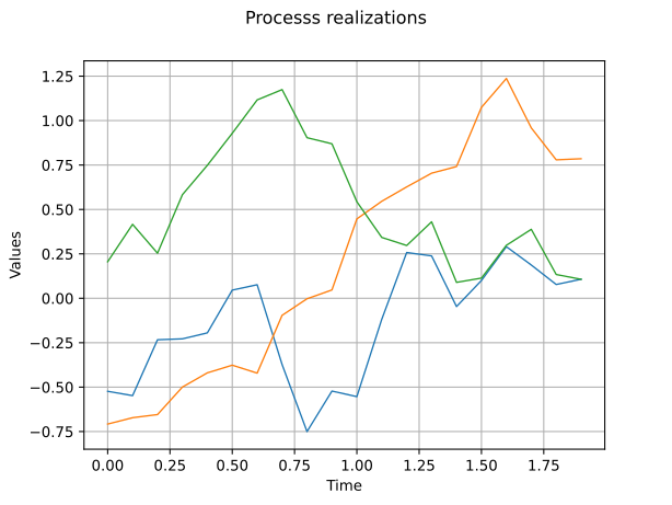
Eventually we draw some realizations of the Gaussian process.

sample = process.getSample(n_real)
graph = sample.drawMarginal(0)
graph.setTitle("Processs realizations")
view = otv.View(graph)

Display all figures.

otv.View.ShowAll()