FunctionalChaosRandomVector¶

class FunctionalChaosRandomVector(*args)¶

Functional chaos random vector.

Allows one to simulate a variable through a chaos decomposition, and retrieve its mean and covariance analytically from the chaos coefficients.

Parameters:

functionalChaosResultFunctionalChaosResult: A result from a functional chaos decomposition.

See also

FunctionalChaosAlgorithm, FunctionalChaosResult

Methods

`asComposedEvent`()	If the random vector can be viewed as the composition of several `ThresholdEvent` objects, this method builds and returns the composition.
`getAntecedent`()	Accessor to the antecedent RandomVector in case of a composite RandomVector.
`getClassName`()	Accessor to the object's name.
`getCovariance`()	Accessor to the covariance of the functional chaos expansion.
`getDescription`()	Accessor to the description of the RandomVector.
`getDimension`()	Accessor to the dimension of the RandomVector.
`getDistribution`()	Accessor to the distribution of the RandomVector.
`getDomain`()	Accessor to the domain of the Event.
`getFrozenRealization`(fixedPoint)	Compute realizations of the RandomVector.
`getFrozenSample`(fixedSample)	Compute realizations of the RandomVector.
`getFunction`()	Accessor to the Function in case of a composite RandomVector.
`getFunctionalChaosResult`()	Accessor to the functional chaos result.
`getId`()	Accessor to the object's id.
`getMarginal`(*args)	Get the random vector corresponding to the $i^{th}$ marginal component(s).
`getMean`()	Accessor to the mean of the functional chaos expansion.
`getName`()	Accessor to the object's name.
`getOperator`()	Accessor to the comparaison operator of the Event.
`getParameter`()	Accessor to the parameter of the distribution.
`getParameterDescription`()	Accessor to the parameter description of the distribution.
`getProcess`()	Get the stochastic process.
`getRealization`()	Compute one realization of the RandomVector.
`getSample`(size)	Compute realizations of the RandomVector.
`getShadowedId`()	Accessor to the object's shadowed id.
`getThreshold`()	Accessor to the threshold of the Event.
`getVisibility`()	Accessor to the object's visibility state.
`hasName`()	Test if the object is named.
`hasVisibleName`()	Test if the object has a distinguishable name.
`isComposite`()	Accessor to know if the RandomVector is a composite one.
`isEvent`()	Whether the random vector is an event.
`setDescription`(description)	Accessor to the description of the RandomVector.
`setName`(name)	Accessor to the object's name.
`setParameter`(parameters)	Accessor to the parameter of the distribution.
`setShadowedId`(id)	Accessor to the object's shadowed id.
`setVisibility`(visible)	Accessor to the object's visibility state.

__init__(*args)¶

asComposedEvent()¶

If the random vector can be viewed as the composition of several ThresholdEvent objects, this method builds and returns the composition. Otherwise throws.

Returns:

composedRandomVector: Composed event.

getAntecedent()¶

Accessor to the antecedent RandomVector in case of a composite RandomVector.

Returns:

antecedentRandomVector: Antecedent RandomVector $\vect{X}$ in case of a CompositeRandomVector such as: $\vect{Y}=f(\vect{X})$ .

getClassName()¶

Accessor to the object’s name.

Returns:

class_namestr: The object class name (object.__class__.__name__).

getCovariance()¶

Accessor to the covariance of the functional chaos expansion.

Let $n_X \in \Nset$ be the dimension of the input random vector, let $n_Y \in \Nset$ be the dimension of the output random vector. and let $P \in \Nset$ be the number of coefficients in the basis. We consider the following functional chaos expansion:

$\widetilde{\vect{Y}} = \sum_{k = 0}^P \vect{a}_k \psi_k(\vect{Z})$

where $\widetilde{\vect{Y}} \in \Rset^{n_Y}$ is the approximation of the output random variable $\vect{Y}$ by the expansion, $\left\{\vect{a}_k \in \Rset^{n_Y}\right\}_{k = 0, ..., P}$ are the coefficients, $\left\{\psi_k: \Rset^{n_X} \rightarrow \Rset\right\}_{k = 0, ..., P}$ are the orthonormal functions in the basis, and $\vect{Z} \in \Rset^{n_X}$ is the standardized random input vector. The previous equation can be equivalently written as follows:

$\widetilde{Y}_i = \sum_{k = 0}^P a_{ki} \psi_k(\vect{Z})$

for $i = 1, ..., n_Y$ where $a_{ki} \in \Rset$ is the $i$ -th component of the $k$ -th coefficient in the expansion:

$\vect{a}_k = \begin{pmatrix}a_{k, 1} \\ \vdots\\ a_{k, n_Y} \end{pmatrix}.$

The covariance matrix of the functional chaos expansion is the matrix $\matcov \in \Rset^{n_Y \times n_Y}$ , where each component is:

$c_{ij} = \Cov{\widetilde{Y}_i, \tilde{Y}_j}$

for $i,j = 1, ..., n_Y$ . The covariance can be computed using the coefficients of the expansion:

$\Cov{\widetilde{Y}_i, \tilde{Y}_j} = \sum_{k = 1}^P a_{ki} a_{jk}$

for $i,j = 1, ..., n_Y$ . This covariance involves all the coefficients, except the first one. The diagonal of the covariance matrix is the marginal variance:

$\Var{\widetilde{Y}_i} = \sum_{k = 1}^P a_{ki}^2$

for $i,j = 1, ..., n_Y$ .

Returns:

covarianceCovarianceMatrix, dimension $n_Y \times n_Y$: The covariance of the functional chaos expansion.

Examples

>>> from openturns.usecases import ishigami_function
>>> import openturns as ot
>>> import math
>>> im = ishigami_function.IshigamiModel()
>>> sampleSize = 1000
>>> inputTrain = im.distributionX.getSample(sampleSize)
>>> outputTrain = im.model(inputTrain)
>>> multivariateBasis = ot.OrthogonalProductPolynomialFactory([im.X1, im.X2, im.X3])
>>> selectionAlgorithm = ot.LeastSquaresMetaModelSelectionFactory()
>>> projectionStrategy = ot.LeastSquaresStrategy(selectionAlgorithm)
>>> totalDegree = 10
>>> enumerateFunction = multivariateBasis.getEnumerateFunction()
>>> basisSize = enumerateFunction.getBasisSizeFromTotalDegree(totalDegree)
>>> adaptiveStrategy = ot.FixedStrategy(multivariateBasis, basisSize)
>>> chaosAlgo = ot.FunctionalChaosAlgorithm(
...     inputTrain, outputTrain, im.distributionX, adaptiveStrategy, projectionStrategy
... )
>>> chaosAlgo.run()
>>> chaosResult = chaosAlgo.getResult()
>>> randomVector = ot.FunctionalChaosRandomVector(chaosResult)
>>> covarianceMatrix = randomVector.getCovariance()
>>> covarianceMatrix = randomVector.getCovariance()
>>> print('covarianceMatrix=', covarianceMatrix[0, 0])
covarianceMatrix= 13.8...
>>> outputDimension = outputTrain.getDimension()
>>> stdDev = ot.Point([math.sqrt(covarianceMatrix[i, i]) for i in range(outputDimension)])
>>> print('stdDev=', stdDev[0])
stdDev= 3.72...

getDescription()¶

Accessor to the description of the RandomVector.

Returns:

descriptionDescription: Describes the components of the RandomVector.

getDimension()¶

Accessor to the dimension of the RandomVector.

Returns:

dimensionpositive int: Dimension of the RandomVector.

getDistribution()¶

Accessor to the distribution of the RandomVector.

Returns:

distributionDistribution: Distribution of the considered UsualRandomVector.

Examples

>>> import openturns as ot
>>> distribution = ot.Normal([0.0, 0.0], [1.0, 1.0], ot.CorrelationMatrix(2))
>>> randomVector = ot.RandomVector(distribution)
>>> ot.RandomGenerator.SetSeed(0)
>>> print(randomVector.getDistribution())
Normal(mu = [0,0], sigma = [1,1], R = [[ 1 0 ]
 [ 0 1 ]])

getDomain()¶

Accessor to the domain of the Event.

Returns:

domainDomain: Describes the domain of an event.

getFrozenRealization(fixedPoint)¶

Compute realizations of the RandomVector.

In the case of a CompositeRandomVector or an event of some kind, this method returns the value taken by the random vector if the root cause takes the value given as argument.

Parameters:

fixedPointPoint: Point chosen as the root cause of the random vector.

Returns:

realizationPoint: The realization corresponding to the chosen root cause.

See also

getRealization
getFrozenSample

Examples

>>> import openturns as ot
>>> distribution = ot.Normal()
>>> randomVector = ot.RandomVector(distribution)
>>> f = ot.SymbolicFunction('x', 'x')
>>> compositeRandomVector = ot.CompositeRandomVector(f, randomVector)
>>> event = ot.ThresholdEvent(compositeRandomVector, ot.Less(), 0.0)
>>> print(event.getFrozenRealization([0.2]))
[0]
>>> print(event.getFrozenRealization([-0.1]))
[1]

getFrozenSample(fixedSample)¶

Compute realizations of the RandomVector.

In the case of a CompositeRandomVector or an event of some kind, this method returns the different values taken by the random vector when the root cause takes the values given as argument.

Parameters:

fixedSampleSample: Sample of root causes of the random vector.

Returns:

sampleSample: Sample of the realizations corresponding to the chosen root causes.

See also

getSample
getFrozenRealization

Examples

>>> import openturns as ot
>>> distribution = ot.Normal()
>>> randomVector = ot.RandomVector(distribution)
>>> f = ot.SymbolicFunction('x', 'x')
>>> compositeRandomVector = ot.CompositeRandomVector(f, randomVector)
>>> event = ot.ThresholdEvent(compositeRandomVector, ot.Less(), 0.0)
>>> print(event.getFrozenSample([[0.2], [-0.1]]))
    [ y0 ]
0 : [ 0  ]
1 : [ 1  ]

getFunction()¶

Accessor to the Function in case of a composite RandomVector.

Returns:

functionFunction: Function used to define a CompositeRandomVector as the image through this function of the antecedent $\vect{X}$ : $\vect{Y}=f(\vect{X})$ .

getFunctionalChaosResult()¶

Accessor to the functional chaos result.

Returns:

functionalChaosResultFunctionalChaosResult: The result from a functional chaos decomposition.

getId()¶

Accessor to the object’s id.

Returns:

idint: Internal unique identifier.

getMarginal(*args)¶

Get the random vector corresponding to the $i^{th}$ marginal component(s).

Parameters:

iint or list of ints, $0\leq i < dim$: Indicates the component(s) concerned. $dim$ is the dimension of the RandomVector.

Returns:

vectorRandomVector: RandomVector restricted to the concerned components.

Notes

Let’s note $\vect{Y}=\Tr{(Y_1,\dots,Y_n)}$ a random vector and $I \in [1,n]$ a set of indices. If $\vect{Y}$ is a UsualRandomVector, the subvector is defined by $\tilde{\vect{Y}}=\Tr{(Y_i)}_{i \in I}$ . If $\vect{Y}$ is a CompositeRandomVector, defined by $\vect{Y}=f(\vect{X})$ with $f=(f_1,\dots,f_n)$ , $f_i$ some scalar functions, the subvector is $\tilde{\vect{Y}}=(f_i(\vect{X}))_{i \in I}$ .

Examples

>>> import openturns as ot
>>> distribution = ot.Normal([0.0, 0.0], [1.0, 1.0], ot.CorrelationMatrix(2))
>>> randomVector = ot.RandomVector(distribution)
>>> ot.RandomGenerator.SetSeed(0)
>>> print(randomVector.getMarginal(1).getRealization())
[0.608202]
>>> print(randomVector.getMarginal(1).getDistribution())
Normal(mu = 0, sigma = 1)

getMean()¶

Accessor to the mean of the functional chaos expansion.

Let $n_X \in \Nset$ be the dimension of the input random vector, let $n_Y \in \Nset$ be the dimension of the output random vector. and let $P \in \Nset$ be the number of coefficients in the basis. We consider the following functional chaos expansion:

$\widetilde{\vect{Y}} = \sum_{k = 0}^P \vect{a}_k \psi_k(\vect{Z})$

where $\widetilde{\vect{Y}} \in \Rset^{n_Y}$ is the approximation of the output random variable $\vect{Y}$ by the expansion, $\left\{\vect{a}_k \in \Rset^{n_Y}\right\}_{k = 0, ..., P}$ are the coefficients, $\left\{\psi_k: \Rset^{n_X} \rightarrow \Rset\right\}_{k = 0, ..., P}$ are the orthonormal functions in the basis, and $\vect{Z} \in \Rset^{n_X}$ is the standardized random input vector. The previous equation can be equivalently written as follows:

$\widetilde{Y}_i = \sum_{k = 0}^P a_{ki} \psi_k(\vect{Z})$

for $i = 1, ..., n_Y$ where $a_{ki} \in \Rset$ is the $i$ -th component of the $k$ -th coefficient in the expansion:

$\vect{a}_k = \begin{pmatrix}a_{k, 1} \\ \vdots\\ a_{k, n_Y} \end{pmatrix}.$

The mean of the functional chaos expansion is the first coefficient in the expansion:

$\Expect{\widetilde{Y}_i} = a_{i,0}$

for $i = 1, ..., n_Y$ .

Returns:

meanPoint, dimension $n_Y$: The mean of the functional chaos expansion.

Examples

>>> from openturns.usecases import ishigami_function
>>> import openturns as ot
>>> im = ishigami_function.IshigamiModel()
>>> sampleSize = 1000
>>> inputTrain = im.distributionX.getSample(sampleSize)
>>> outputTrain = im.model(inputTrain)
>>> multivariateBasis = ot.OrthogonalProductPolynomialFactory([im.X1, im.X2, im.X3])
>>> selectionAlgorithm = ot.LeastSquaresMetaModelSelectionFactory()
>>> projectionStrategy = ot.LeastSquaresStrategy(selectionAlgorithm)
>>> totalDegree = 10
>>> enumerateFunction = multivariateBasis.getEnumerateFunction()
>>> basisSize = enumerateFunction.getBasisSizeFromTotalDegree(totalDegree)
>>> adaptiveStrategy = ot.FixedStrategy(multivariateBasis, basisSize)
>>> chaosAlgo = ot.FunctionalChaosAlgorithm(
...     inputTrain, outputTrain, im.distributionX, adaptiveStrategy, projectionStrategy
... )
>>> chaosAlgo.run()
>>> chaosResult = chaosAlgo.getResult()
>>> randomVector = ot.FunctionalChaosRandomVector(chaosResult)
>>> mean = randomVector.getMean()
>>> print('mean=', mean[0])
mean= 3.50...

getName()¶

Accessor to the object’s name.

Returns:

namestr: The name of the object.

getOperator()¶

Accessor to the comparaison operator of the Event.

Returns:

operatorComparisonOperator: Comparaison operator used to define the RandomVector.

getParameter()¶

Accessor to the parameter of the distribution.

Returns:

parameterPoint: Parameter values.

getParameterDescription()¶

Accessor to the parameter description of the distribution.

Returns:

descriptionDescription: Parameter names.

getProcess()¶

Get the stochastic process.

Returns:

processProcess: Stochastic process used to define the RandomVector.

getRealization()¶

Compute one realization of the RandomVector.

Returns:

aRealizationPoint: Sequence of values randomly determined from the RandomVector definition. In the case of an event: one realization of the event (considered as a Bernoulli variable) which is a boolean value (1 for the realization of the event and 0 else).

See also

getSample

Examples

>>> import openturns as ot
>>> distribution = ot.Normal([0.0, 0.0], [1.0, 1.0], ot.CorrelationMatrix(2))
>>> randomVector = ot.RandomVector(distribution)
>>> ot.RandomGenerator.SetSeed(0)
>>> print(randomVector.getRealization())
[0.608202,-1.26617]
>>> print(randomVector.getRealization())
[-0.438266,1.20548]

getSample(size)¶

Compute realizations of the RandomVector.

Parameters:

nint, $n \geq 0$: Number of realizations needed.

Returns:

realizationsSample: n sequences of values randomly determined from the RandomVector definition. In the case of an event: n realizations of the event (considered as a Bernoulli variable) which are boolean values (1 for the realization of the event and 0 else).

See also

getRealization

Examples

>>> import openturns as ot
>>> distribution = ot.Normal([0.0, 0.0], [1.0, 1.0], ot.CorrelationMatrix(2))
>>> randomVector = ot.RandomVector(distribution)
>>> ot.RandomGenerator.SetSeed(0)
>>> print(randomVector.getSample(3))
    [ X0        X1        ]
0 : [  0.608202 -1.26617  ]
1 : [ -0.438266  1.20548  ]
2 : [ -2.18139   0.350042 ]

getShadowedId()¶

Accessor to the object’s shadowed id.

Returns:

idint: Internal unique identifier.

getThreshold()¶

Accessor to the threshold of the Event.

Returns:

thresholdfloat: Threshold of the RandomVector.

getVisibility()¶

Accessor to the object’s visibility state.

Returns:

visiblebool: Visibility flag.

hasName()¶

Test if the object is named.

Returns:

hasNamebool: True if the name is not empty.

hasVisibleName()¶

Test if the object has a distinguishable name.

Returns:

hasVisibleNamebool: True if the name is not empty and not the default one.

isComposite()¶

Accessor to know if the RandomVector is a composite one.

Returns:

isCompositebool: Indicates if the RandomVector is of type Composite or not.

isEvent()¶

Whether the random vector is an event.

Returns:

isEventbool: Whether it takes it values in {0, 1}.

setDescription(description)¶

Accessor to the description of the RandomVector.

Parameters:

descriptionstr or sequence of str: Describes the components of the RandomVector.

setName(name)¶

Accessor to the object’s name.

Parameters:

namestr: The name of the object.

setParameter(parameters)¶

Accessor to the parameter of the distribution.

Parameters:

parametersequence of float: Parameter values.

setShadowedId(id)¶

Accessor to the object’s shadowed id.

Parameters:

idint: Internal unique identifier.

setVisibility(visible)¶

Accessor to the object’s visibility state.

Parameters:

visiblebool: Visibility flag.

Examples using the class¶

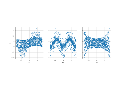
Create a polynomial chaos for the Ishigami function: a quick start guide to polynomial chaos

OpenTURNS

An Open source initiative for the Treatment of Uncertainties, Risks'N Statistics

Table of Contents

Previous topic

Next topic

This Page

FunctionalChaosRandomVector¶

Examples using the class¶