Draw multidimensional functions, distributions and events

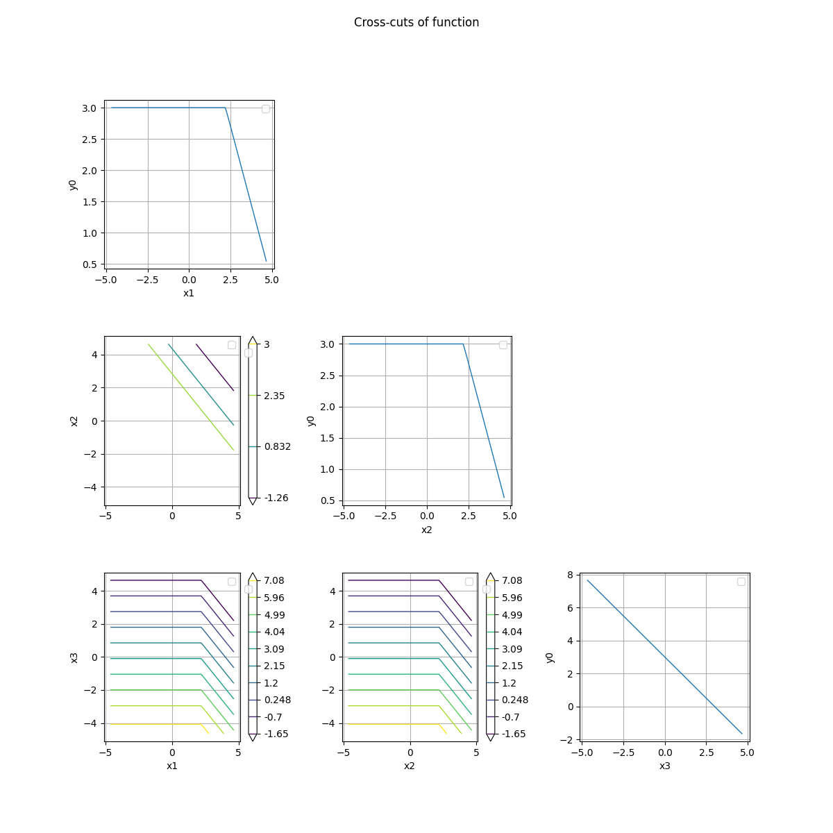
This example shows how to represent multidimensional functions, distributions and events. When 2D plots are to draw, contours are used. We use 2D cross-sections to represent multidimensional objects when required, which leads to cross-cuts representations.

import otbenchmark as otb
import openturns.viewer as otv
import matplotlib.pyplot as plt

problem = otb.ReliabilityProblem33()

event = problem.getEvent()
g = event.getFunction()

Compute the bounds of the domain

inputVector = event.getAntecedent()
distribution = inputVector.getDistribution()

inputDimension = distribution.getDimension()
inputDimension

3

alpha = 1 - 1.0e-5

bounds, marginalProb = distribution.computeMinimumVolumeIntervalWithMarginalProbability(
    alpha
)

referencePoint = distribution.getMean()
referencePoint

class=Point name=Unnamed dimension=3 values=[0,0,0]

crossCut = otb.CrossCutFunction(g, referencePoint)
fig = crossCut.draw(bounds)
# Remove the legend labels because there
# are too many for such a small figure
for ax in fig.axes:
    ax.legend("")
# Increase space between sub-figures so that
# there are no overlap
plt.subplots_adjust(hspace=0.4, wspace=0.4)

Plot cross-cuts of the distribution

crossCut = otb.CrossCutDistribution(distribution)

fig = crossCut.drawMarginalPDF()
# Remove the legend labels because there
# are too many for such a small figure
for ax in fig.axes:
    ax.legend("")
# Increase space between sub-figures so that
# there are no overlap
plt.subplots_adjust(hspace=0.4, wspace=0.4)

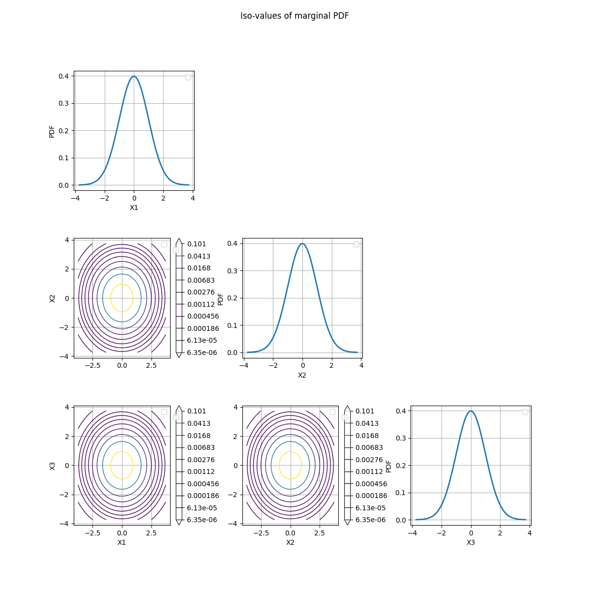
The correct way to represent cross-cuts of a distribution is to draw the contours of the PDF of the conditional distribution.

fig = crossCut.drawConditionalPDF(referencePoint)
# Remove the legend labels because there
# are too many for such a small figure
for ax in fig.axes:
    ax.legend("")
# Increase space between sub-figures so that
# there are no overlap
plt.subplots_adjust(hspace=0.4, wspace=0.4)

Descr =  1 0
Descr =  2 0
Descr =  2 1

inputVector = event.getAntecedent()
event = problem.getEvent()
g = event.getFunction()

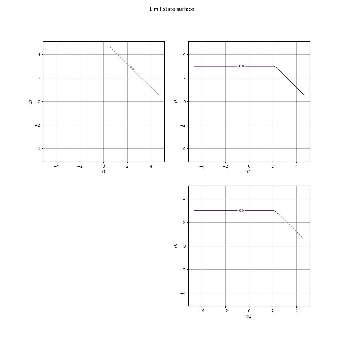
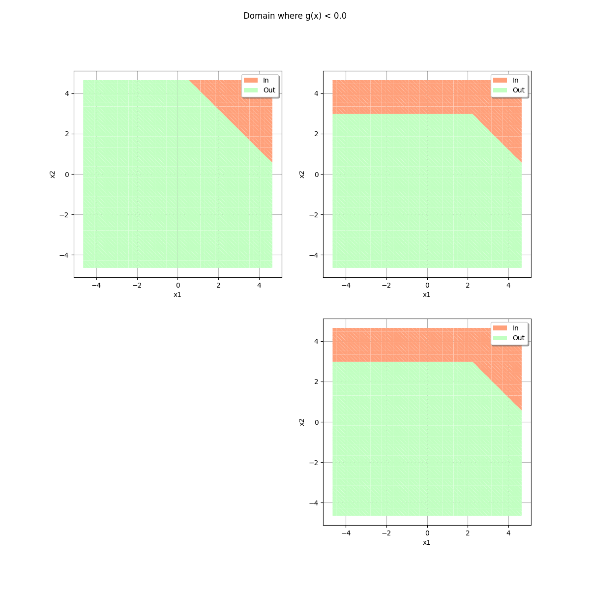
drawEvent = otb.DrawEvent(event)

_ = drawEvent.drawLimitState(bounds)

In the following figure, we present the cross-cuts of samples with size equal to 500. These are three different samples, each of which is plotted with the drawSampleCrossCut method. For each cross-cut plot (i,j), the current implementation uses the marginal bivariate distribution, then generates a sample from this distribution. A more rigorous method would draw the conditional distribution, but this might reduce the performance in general. See https://github.com/mbaudin47/otbenchmark/issues/47 for details.

sampleSize = 500
_ = drawEvent.drawSample(sampleSize)

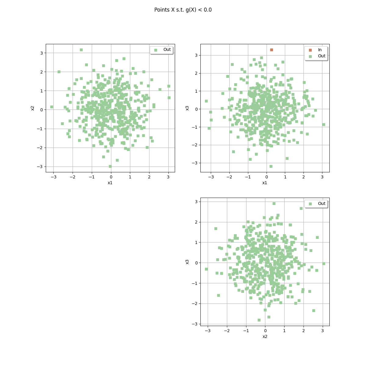
_ = drawEvent.fillEvent(bounds)

otv.View.ShowAll()