R-S analysis and 2D graphics

The objective of this example is to present the R-S problem. We also present graphic elements for the visualization of the limit state surface in 2 dimensions.

import openturns as ot
import openturns.viewer as otv
import otbenchmark as otb

problem = otb.RminusSReliability()

event = problem.getEvent()
g = event.getFunction()

problem.getProbability()

0.07864960352514257

Create the Monte-Carlo algorithm

algoProb = ot.ProbabilitySimulationAlgorithm(event)
algoProb.setMaximumOuterSampling(1000)
algoProb.setMaximumCoefficientOfVariation(0.01)
algoProb.run()

Get the results

resultAlgo = algoProb.getResult()
neval = g.getEvaluationCallsNumber()
print("Number of function calls = %d" % (neval))
pf = resultAlgo.getProbabilityEstimate()
print("Failure Probability = %.4f" % (pf))
level = 0.95
c95 = resultAlgo.getConfidenceLength(level)
pmin = pf - 0.5 * c95
pmax = pf + 0.5 * c95
print("%.1f %% confidence interval :[%.4f,%.4f] " % (level * 100, pmin, pmax))

Number of function calls = 1000
Failure Probability = 0.0880
95.0 % confidence interval :[0.0704,0.1056]

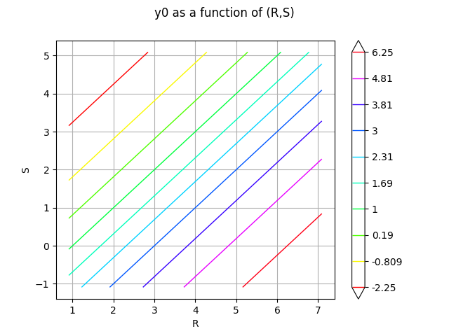
Plot the contours of the function

inputVector = event.getAntecedent()
distribution = inputVector.getDistribution()

R = distribution.getMarginal(0)
S = distribution.getMarginal(1)

alphaMin = 0.001
alphaMax = 1 - alphaMin
lowerBound = ot.Point([R.computeQuantile(alphaMin)[0], S.computeQuantile(alphaMin)[0]])
upperBound = ot.Point([R.computeQuantile(alphaMax)[0], S.computeQuantile(alphaMax)[0]])

nbPoints = [100, 100]
_ = otv.View(g.draw(lowerBound, upperBound, nbPoints))

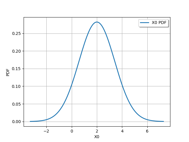
Y = R - S
Y

Normal

• name=Normal
• dimension=1
• weight=1
• range=]-inf (-8.81962), (12.8196) +inf[
• description=[X0]
• isParallel=true
• isCopula=false

_ = otv.View(Y.drawPDF())

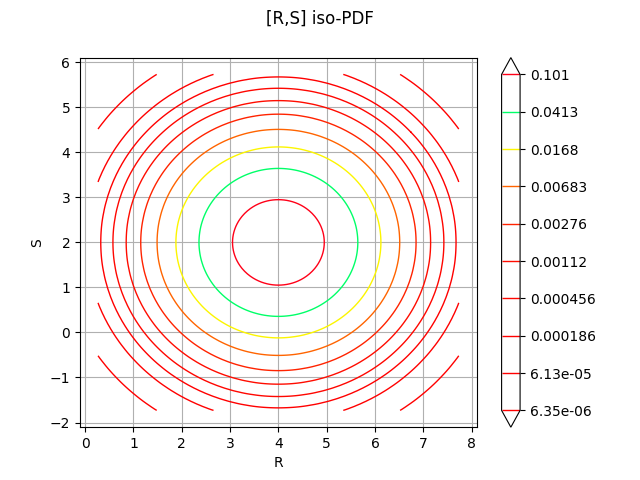
Print the iso-values of the distribution

_ = otv.View(distribution.drawPDF())

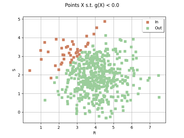
Visualise the safe and unsafe regions on a sample

sampleSize = 500

drawEvent = otb.DrawEvent(event)

cloud = drawEvent.drawSampleCrossCut(sampleSize)
_ = otv.View(cloud)

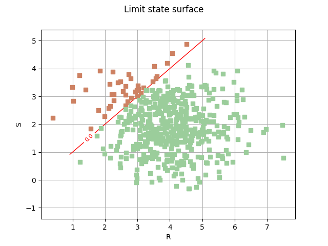
Draw the limit state surface

bounds = ot.Interval(lowerBound, upperBound)
bounds

class=Interval name=Unnamed dimension=2 lower bound=class=Point name=Unnamed dimension=2 values=[0.909768,-1.09023] upper bound=class=Point name=Unnamed dimension=2 values=[7.09023,5.09023] finite lower bound=[1,1] finite upper bound=[1,1]

graph = drawEvent.drawLimitStateCrossCut(bounds)
graph.add(cloud)
_ = otv.View(graph)

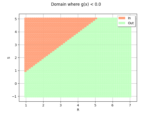
Fill the event domain with a color

domain = drawEvent.fillEventCrossCut(bounds)
_ = otv.View(domain)

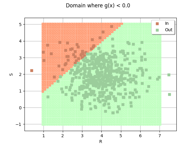
domain.setLegends(["", ""])
domain.add(cloud)
_ = otv.View(domain)

otv.View.ShowAll()