RP57 analysis and 2D graphics

The objective of this example is to present problem 57 of the BBRC. We also present graphic elements for the visualization of the limit state surface in 2 dimensions.

import openturns as ot
import openturns.viewer as otv
import otbenchmark as otb

problem = otb.ReliabilityProblem57()
print(problem)

name = RP57
event = class=ThresholdEventImplementation antecedent=class=CompositeRandomVector function=class=Function name=Unnamed implementation=class=FunctionImplementation name=Unnamed description=[x1,x2,gsys] evaluationImplementation=class=SymbolicEvaluation name=Unnamed inputVariablesNames=[x1,x2] outputVariablesNames=[gsys] formulas=[var g1 := -x1^2 + x2^3 + 3;var g2 := 2 - x1 - 8 * x2;var g3 := (x1 + 3)^2 + (x2 + 3)^2 - 4;gsys := min(max(g1, g2), g3) ] gradientImplementation=class=SymbolicGradient name=Unnamed evaluation=class=SymbolicEvaluation name=Unnamed inputVariablesNames=[x1,x2] outputVariablesNames=[gsys] formulas=[var g1 := -x1^2 + x2^3 + 3;var g2 := 2 - x1 - 8 * x2;var g3 := (x1 + 3)^2 + (x2 + 3)^2 - 4;gsys := min(max(g1, g2), g3) ] hessianImplementation=class=SymbolicHessian name=Unnamed evaluation=class=SymbolicEvaluation name=Unnamed inputVariablesNames=[x1,x2] outputVariablesNames=[gsys] formulas=[var g1 := -x1^2 + x2^3 + 3;var g2 := 2 - x1 - 8 * x2;var g3 := (x1 + 3)^2 + (x2 + 3)^2 - 4;gsys := min(max(g1, g2), g3) ] antecedent=class=UsualRandomVector distribution=class=JointDistribution name=JointDistribution dimension=2 copula=class=IndependentCopula name=IndependentCopula dimension=2 marginal[0]=class=Normal name=Normal dimension=1 mean=class=Point name=Unnamed dimension=1 values=[0] sigma=class=Point name=Unnamed dimension=1 values=[1] correlationMatrix=class=CorrelationMatrix dimension=1 implementation=class=MatrixImplementation name=Unnamed rows=1 columns=1 values=[1] marginal[1]=class=Normal name=Normal dimension=1 mean=class=Point name=Unnamed dimension=1 values=[0] sigma=class=Point name=Unnamed dimension=1 values=[1] correlationMatrix=class=CorrelationMatrix dimension=1 implementation=class=MatrixImplementation name=Unnamed rows=1 columns=1 values=[1] operator=class=Less name=Unnamed threshold=0
probability = 0.0284

event = problem.getEvent()
g = event.getFunction()

problem.getProbability()

0.0284

Create the Monte-Carlo algorithm

algoProb = ot.ProbabilitySimulationAlgorithm(event)
algoProb.setMaximumOuterSampling(1000)
algoProb.setMaximumCoefficientOfVariation(0.01)
algoProb.run()

Get the results

resultAlgo = algoProb.getResult()
neval = g.getEvaluationCallsNumber()
print("Number of function calls = %d" % (neval))
pf = resultAlgo.getProbabilityEstimate()
print("Failure Probability = %.4f" % (pf))
level = 0.95
c95 = resultAlgo.getConfidenceLength(level)
pmin = pf - 0.5 * c95
pmax = pf + 0.5 * c95
print("%.1f %% confidence interval :[%.4f,%.4f] " % (level * 100, pmin, pmax))

Number of function calls = 1000
Failure Probability = 0.0360
95.0 % confidence interval :[0.0245,0.0475]

Compute the bounds of the domain

inputVector = event.getAntecedent()
distribution = inputVector.getDistribution()
X1 = distribution.getMarginal(0)
X2 = distribution.getMarginal(1)
alphaMin = 0.00001
alphaMax = 1 - alphaMin
lowerBound = ot.Point(
    [X1.computeQuantile(alphaMin)[0], X2.computeQuantile(alphaMin)[0]]
)
upperBound = ot.Point(
    [X1.computeQuantile(alphaMax)[0], X2.computeQuantile(alphaMax)[0]]
)

nbPoints = [100, 100]
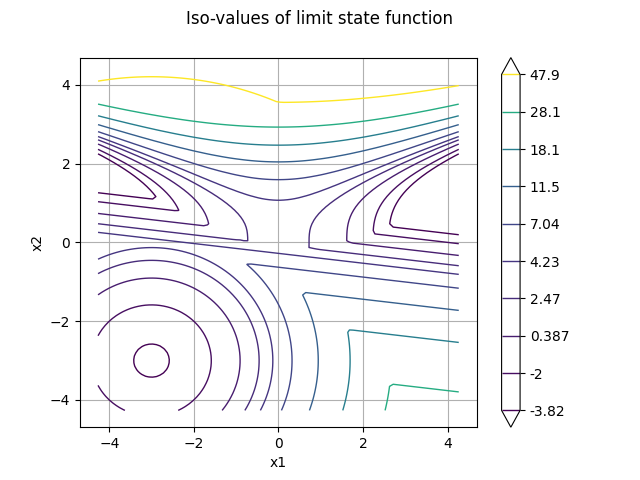
graph = g.draw(lowerBound, upperBound, nbPoints)
graph.setTitle("Iso-values of limit state function")
_ = otv.View(graph)

Print the iso-values of the distribution

distribution.drawPDF()

class=Graph name=pdf as a function of (X1,X2) implementation=class=GraphImplementation name=pdf as a function of (X1,X2) title=[X1,X2] iso-PDF xTitle=X1 yTitle=X2 axes=ON grid=ON legendposition=upper left legendFontSize=1 drawables=[class=Drawable name=Unnamed implementation=class=Contour name=Unnamed x=class=Sample name=Unnamed implementation=class=SampleImplementation name=Unnamed size=129 dimension=1 data=[[-3.73116],[-3.67286],[-3.61456],[-3.55626],[-3.49796],[-3.43966],[-3.38136],[-3.32306],[-3.26477],[-3.20647],[-3.14817],[-3.08987],[-3.03157],[-2.97327],[-2.91497],[-2.85667],[-2.79837],[-2.74007],[-2.68177],[-2.62347],[-2.56517],[-2.50687],[-2.44857],[-2.39027],[-2.33198],[-2.27368],[-2.21538],[-2.15708],[-2.09878],[-2.04048],[-1.98218],[-1.92388],[-1.86558],[-1.80728],[-1.74898],[-1.69068],[-1.63238],[-1.57408],[-1.51578],[-1.45748],[-1.39919],[-1.34089],[-1.28259],[-1.22429],[-1.16599],[-1.10769],[-1.04939],[-0.991089],[-0.93279],[-0.874491],[-0.816191],[-0.757892],[-0.699593],[-0.641293],[-0.582994],[-0.524694],[-0.466395],[-0.408096],[-0.349796],[-0.291497],[-0.233198],[-0.174898],[-0.116599],[-0.0582994],[0],[0.0582994],[0.116599],[0.174898],[0.233198],[0.291497],[0.349796],[0.408096],[0.466395],[0.524694],[0.582994],[0.641293],[0.699593],[0.757892],[0.816191],[0.874491],[0.93279],[0.991089],[1.04939],[1.10769],[1.16599],[1.22429],[1.28259],[1.34089],[1.39919],[1.45748],[1.51578],[1.57408],[1.63238],[1.69068],[1.74898],[1.80728],[1.86558],[1.92388],[1.98218],[2.04048],[2.09878],[2.15708],[2.21538],[2.27368],[2.33198],[2.39027],[2.44857],[2.50687],[2.56517],[2.62347],[2.68177],[2.74007],[2.79837],[2.85667],[2.91497],[2.97327],[3.03157],[3.08987],[3.14817],[3.20647],[3.26477],[3.32306],[3.38136],[3.43966],[3.49796],[3.55626],[3.61456],[3.67286],[3.73116]] y=class=Sample name=Unnamed implementation=class=SampleImplementation name=Unnamed size=129 dimension=1 data=[[-3.73116],[-3.67286],[-3.61456],[-3.55626],[-3.49796],[-3.43966],[-3.38136],[-3.32306],[-3.26477],[-3.20647],[-3.14817],[-3.08987],[-3.03157],[-2.97327],[-2.91497],[-2.85667],[-2.79837],[-2.74007],[-2.68177],[-2.62347],[-2.56517],[-2.50687],[-2.44857],[-2.39027],[-2.33198],[-2.27368],[-2.21538],[-2.15708],[-2.09878],[-2.04048],[-1.98218],[-1.92388],[-1.86558],[-1.80728],[-1.74898],[-1.69068],[-1.63238],[-1.57408],[-1.51578],[-1.45748],[-1.39919],[-1.34089],[-1.28259],[-1.22429],[-1.16599],[-1.10769],[-1.04939],[-0.991089],[-0.93279],[-0.874491],[-0.816191],[-0.757892],[-0.699593],[-0.641293],[-0.582994],[-0.524694],[-0.466395],[-0.408096],[-0.349796],[-0.291497],[-0.233198],[-0.174898],[-0.116599],[-0.0582994],[0],[0.0582994],[0.116599],[0.174898],[0.233198],[0.291497],[0.349796],[0.408096],[0.466395],[0.524694],[0.582994],[0.641293],[0.699593],[0.757892],[0.816191],[0.874491],[0.93279],[0.991089],[1.04939],[1.10769],[1.16599],[1.22429],[1.28259],[1.34089],[1.39919],[1.45748],[1.51578],[1.57408],[1.63238],[1.69068],[1.74898],[1.80728],[1.86558],[1.92388],[1.98218],[2.04048],[2.09878],[2.15708],[2.21538],[2.27368],[2.33198],[2.39027],[2.44857],[2.50687],[2.56517],[2.62347],[2.68177],[2.74007],[2.79837],[2.85667],[2.91497],[2.97327],[3.03157],[3.08987],[3.14817],[3.20647],[3.26477],[3.32306],[3.38136],[3.43966],[3.49796],[3.55626],[3.61456],[3.67286],[3.73116]] levels=class=Point name=Unnamed dimension=10 values=[6.35446e-06,6.13238e-05,0.000186025,0.000456309,0.0011193,0.0027643,0.00682692,0.0168316,0.041287,0.101447] labels=[6.35446e-06,6.13238e-05,0.000186025,0.000456309,0.0011193,0.0027643,0.00682692,0.0168316,0.041287,0.101447] show labels=false isFilled=false colorBarPosition=right isVminUsed=false vmin=0 isVmaxUsed=false vmax=0 colorMap=hsv alpha=1 norm=linear extend=both hatches=[] derived from class=DrawableImplementation name=Unnamed legend= data=class=Sample name=Unnamed implementation=class=SampleImplementation name=Unnamed size=16641 dimension=1 data=[[1.43141e-07],[1.77622e-07],[2.19661e-07],...,[2.19661e-07],[1.77622e-07],[1.43141e-07]] color=#1f77b4 isColorExplicitlySet=true fillStyle=solid lineStyle=solid pointStyle=plus lineWidth=1]

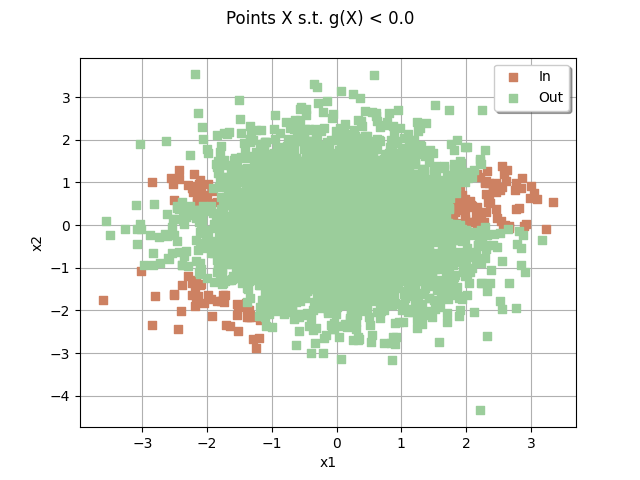
sampleSize = 5000
drawEvent = otb.DrawEvent(event)

cloud = drawEvent.drawSampleCrossCut(sampleSize)
_ = otv.View(cloud)

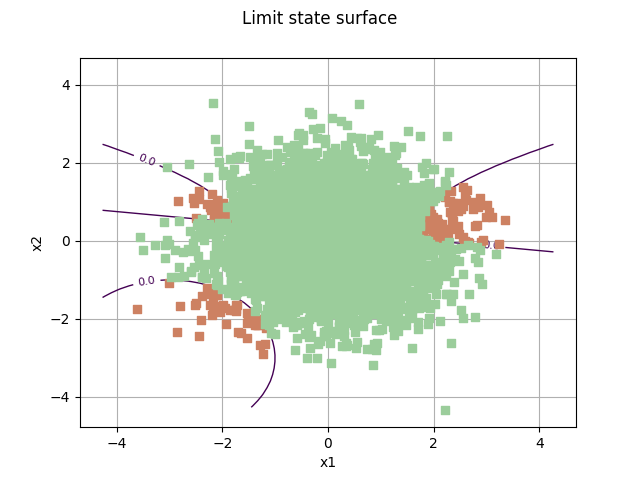
Draw the limit state surface

bounds = ot.Interval(lowerBound, upperBound)
bounds

class=Interval name=Unnamed dimension=2 lower bound=class=Point name=Unnamed dimension=2 values=[-4.26489,-4.26489] upper bound=class=Point name=Unnamed dimension=2 values=[4.26489,4.26489] finite lower bound=[1,1] finite upper bound=[1,1]

graph = drawEvent.drawLimitStateCrossCut(bounds)
graph.add(cloud)
_ = otv.View(graph)

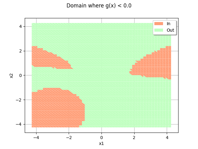
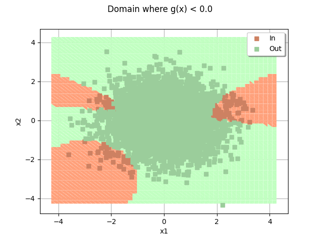
domain = drawEvent.fillEventCrossCut(bounds)
_ = otv.View(domain)

domain.add(cloud)
_ = otv.View(domain)

otv.View.ShowAll()