RP31 analysis and 2D graphics

The objective of this example is to present problem 31 of the BBRC. We also present graphic elements for the visualization of the limit state surface in 2 dimensions.

import openturns as ot
import openturns.viewer as otv
import otbenchmark as otb

problem = otb.ReliabilityProblem31()
print(problem)

name = RP31
event = class=ThresholdEventImplementation antecedent=class=CompositeRandomVector function=class=Function name=Unnamed implementation=class=FunctionImplementation name=Unnamed description=[x1,x2,y0] evaluationImplementation=class=SymbolicEvaluation name=Unnamed inputVariablesNames=[x1,x2] outputVariablesNames=[y0] formulas=[2 - x2 + 256 * x1^4] gradientImplementation=class=SymbolicGradient name=Unnamed evaluation=class=SymbolicEvaluation name=Unnamed inputVariablesNames=[x1,x2] outputVariablesNames=[y0] formulas=[2 - x2 + 256 * x1^4] hessianImplementation=class=SymbolicHessian name=Unnamed evaluation=class=SymbolicEvaluation name=Unnamed inputVariablesNames=[x1,x2] outputVariablesNames=[y0] formulas=[2 - x2 + 256 * x1^4] antecedent=class=UsualRandomVector distribution=class=JointDistribution name=JointDistribution dimension=2 copula=class=IndependentCopula name=IndependentCopula dimension=2 marginal[0]=class=Normal name=Normal dimension=1 mean=class=Point name=Unnamed dimension=1 values=[0] sigma=class=Point name=Unnamed dimension=1 values=[1] correlationMatrix=class=CorrelationMatrix dimension=1 implementation=class=MatrixImplementation name=Unnamed rows=1 columns=1 values=[1] marginal[1]=class=Normal name=Normal dimension=1 mean=class=Point name=Unnamed dimension=1 values=[0] sigma=class=Point name=Unnamed dimension=1 values=[1] correlationMatrix=class=CorrelationMatrix dimension=1 implementation=class=MatrixImplementation name=Unnamed rows=1 columns=1 values=[1] operator=class=Less name=Unnamed threshold=0
probability = 0.003226681209587691

event = problem.getEvent()
g = event.getFunction()

problem.getProbability()

0.003226681209587691

Create the Monte-Carlo algorithm

algoProb = ot.ProbabilitySimulationAlgorithm(event)
algoProb.setMaximumOuterSampling(1000)
algoProb.setMaximumCoefficientOfVariation(0.01)
algoProb.run()

Get the results

resultAlgo = algoProb.getResult()
neval = g.getEvaluationCallsNumber()
print("Number of function calls = %d" % (neval))
pf = resultAlgo.getProbabilityEstimate()
print("Failure Probability = %.4f" % (pf))
level = 0.95
c95 = resultAlgo.getConfidenceLength(level)
pmin = pf - 0.5 * c95
pmax = pf + 0.5 * c95
print("%.1f %% confidence interval :[%.4f,%.4f] " % (level * 100, pmin, pmax))

Number of function calls = 1000
Failure Probability = 0.0030
95.0 % confidence interval :[-0.0004,0.0064]

Compute the bounds of the domain

inputVector = event.getAntecedent()
distribution = inputVector.getDistribution()
X1 = distribution.getMarginal(0)
X2 = distribution.getMarginal(1)
alphaMin = 0.00001
alphaMax = 1 - alphaMin
lowerBound = ot.Point(
    [X1.computeQuantile(alphaMin)[0], X2.computeQuantile(alphaMin)[0]]
)
upperBound = ot.Point(
    [X1.computeQuantile(alphaMax)[0], X2.computeQuantile(alphaMax)[0]]
)

nbPoints = [100, 100]
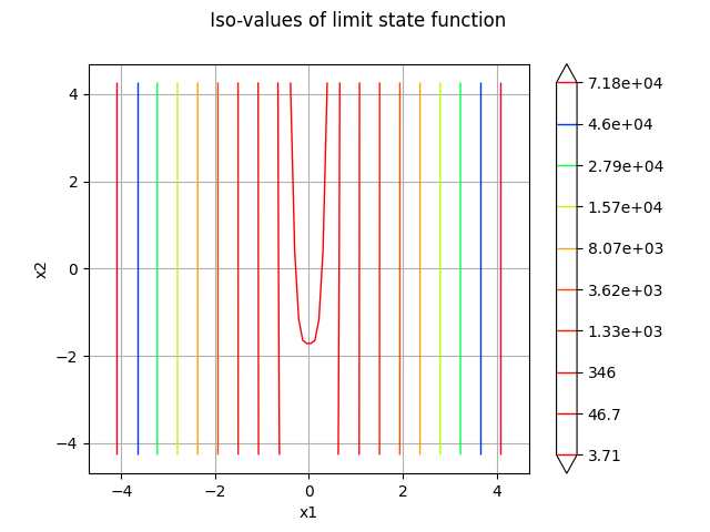
graph = g.draw(lowerBound, upperBound, nbPoints)
graph.setTitle(" Iso-values of limit state function")
_ = otv.View(graph)

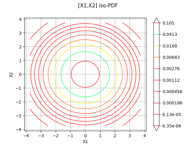
Plot the iso-values of the distribution

_ = otv.View(distribution.drawPDF())

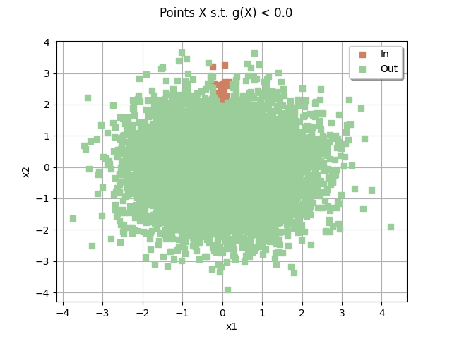
sampleSize = 10000
drawEvent = otb.DrawEvent(event)

cloud = drawEvent.drawSampleCrossCut(sampleSize)
_ = otv.View(cloud)

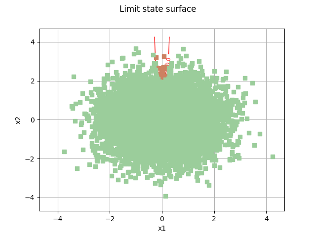
Draw the limit state surface

bounds = ot.Interval(lowerBound, upperBound)

graph = drawEvent.drawLimitStateCrossCut(bounds)
graph.add(cloud)
_ = otv.View(graph)

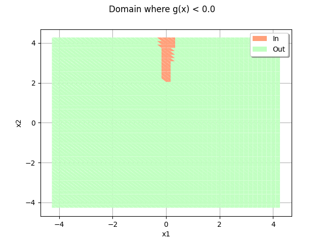
domain = drawEvent.fillEventCrossCut(bounds)
_ = otv.View(domain)

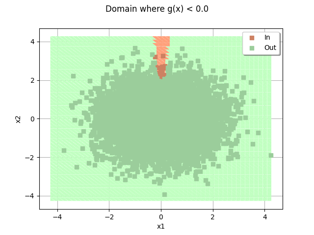
domain.add(cloud)
_ = otv.View(domain)

otv.View.ShowAll()