RP53 analysis and 2D graphics

The objective of this example is to present problem 53 of the BBRC. We also present graphic elements for the visualization of the limit state surface in 2 dimensions.

import openturns as ot
import openturns.viewer as otv
import otbenchmark as otb

problem = otb.ReliabilityProblem53()

event = problem.getEvent()
g = event.getFunction()

problem.getProbability()

0.0313

Create the Monte-Carlo algorithm

algoProb = ot.ProbabilitySimulationAlgorithm(event)
algoProb.setMaximumOuterSampling(1000)
algoProb.setMaximumCoefficientOfVariation(0.01)
algoProb.run()

Get the results

resultAlgo = algoProb.getResult()
neval = g.getEvaluationCallsNumber()
print("Number of function calls = %d" % (neval))
pf = resultAlgo.getProbabilityEstimate()
print("Failure Probability = %.4f" % (pf))
level = 0.95
c95 = resultAlgo.getConfidenceLength(level)
pmin = pf - 0.5 * c95
pmax = pf + 0.5 * c95
print("%.1f %% confidence interval :[%.4f,%.4f] " % (level * 100, pmin, pmax))

Number of function calls = 1000
Failure Probability = 0.0320
95.0 % confidence interval :[0.0211,0.0429]

inputVector = event.getAntecedent()
distribution = inputVector.getDistribution()
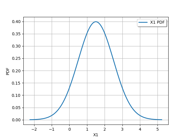
X1 = distribution.getMarginal(0)
X2 = distribution.getMarginal(0)
alpha = 1 - 1.0e-4
bounds, marginalProb = distribution.computeMinimumVolumeIntervalWithMarginalProbability(
    alpha
)

_ = otv.View(X1.drawPDF())

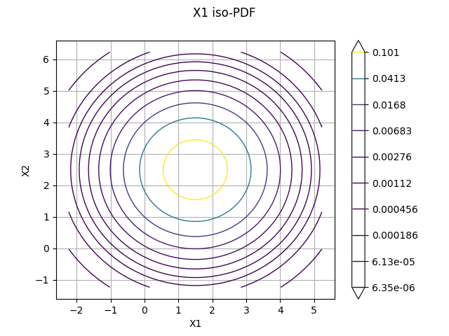
Print the iso-values of the distribution

_ = otv.View(distribution.drawPDF())

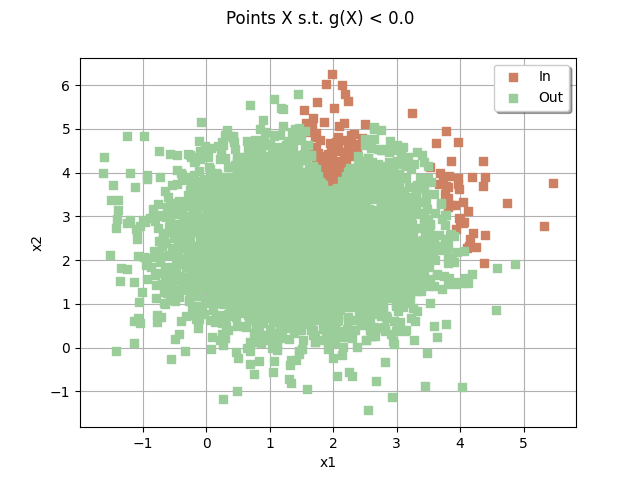
sampleSize = 5000
drawEvent = otb.DrawEvent(event)

cloud = drawEvent.drawSampleCrossCut(sampleSize)
_ = otv.View(cloud)

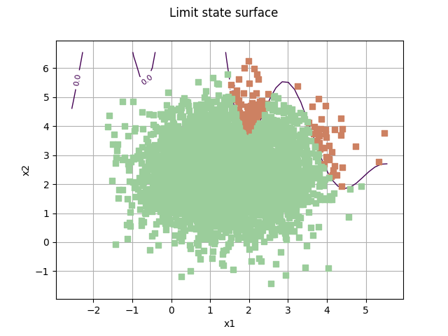
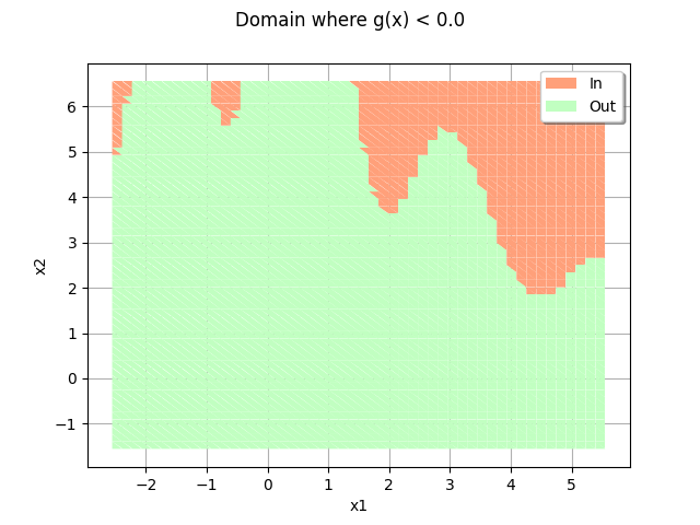
Draw the limit state surface

graph = drawEvent.drawLimitStateCrossCut(bounds)
graph.add(cloud)
_ = otv.View(graph)

domain = drawEvent.fillEventCrossCut(bounds)
_ = otv.View(domain)

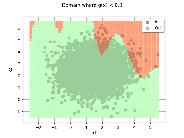
domain.add(cloud)
_ = otv.View(domain)

otv.View.ShowAll()