LeastSquaresStrategy
- class LeastSquaresStrategy(*args)
Least squares strategy for the approximation coefficients.
- Available constructors:
LeastSquaresStrategy(weightedExp)
LeastSquaresStrategy(weightedExp, approxAlgoImpFact)
LeastSquaresStrategy(approxAlgoImpFact)
LeastSquaresStrategy(measure, approxAlgoImpFact)
LeastSquaresStrategy(measure, weightedExp, approxAlgoImpFact)
LeastSquaresStrategy(inputSample, outputSample, approxAlgoImpFact)
LeastSquaresStrategy(inputSample, weights, outputSample, approxAlgoImpFact)
- Parameters:
- weightedExp
WeightedExperiment Experimental design used for the transformed input data. By default the class
MonteCarloExperimentis used.- approxAlgoImpFactApproximationAlgorithmImplementationFactory
The factory that builds the desired
ApproximationAlgorithm. By default the classPenalizedLeastSquaresAlgorithmFactoryis used.- measure
Distribution Distribution
with respect to which the basis is orthonormal. By default, the limit measure defined within the class
WeightedExperimentis used.- inputSample2-d sequence of float
The input random observations
where
is the input of the physical model,
is the input dimension and
is the sample size.
- outputSample2-d sequence of float
The output random observations
where
is the output of the physical model,
is the output dimension and
is the sample size.
- weightssequence of float
Numerical point that are the weights associated to the input sample points such that the corresponding weighted experiment is a good approximation of
. If not precised, all weights are equals to
, where
is the size of the sample.
- weightedExp
Methods
Accessor to the object's name.
Accessor to the coefficients.
Accessor to the design proxy.
Accessor to the experiments.
Accessor to the input sample.
Accessor to the measure.
getName()Accessor to the object's name.
Accessor to the output sample.
Accessor to the relative error.
Accessor to the residual.
Accessor to the weights.
hasName()Test if the object is named.
Get the model selection flag.
Get the least squares flag.
setExperiment(weightedExperiment)Accessor to the design of experiment.
setInputSample(inputSample)Accessor to the input sample.
setMeasure(measure)Accessor to the measure.
setName(name)Accessor to the object's name.
setOutputSample(outputSample)Accessor to the output sample.
setWeights(weights)Accessor to the weights.
Notes
This class is not usable because it has sense only within the
FunctionalChaosAlgorithm: the least squares strategy evaluates the coefficientsof the polynomials decomposition as follows:
where
.
The mean expectation
is approximated by a relation of type:
where is a function
defined as:
In the approximation of the mean expectation, the set I, the points
and the weights
are evaluated from methods implemented in the
WeightedExperiment.- __init__(*args)
- getClassName()
Accessor to the object’s name.
- Returns:
- class_namestr
The object class name (object.__class__.__name__).
- getDesignProxy()
Accessor to the design proxy.
- Parameters:
- designProxy
DesignProxy The design matrix.
- designProxy
- getExperiment()
Accessor to the experiments.
- Returns:
- exp
WeightedExperiment Weighted experiment used to evaluate the coefficients.
- exp
- getMeasure()
Accessor to the measure.
- Returns:
- muDistribution
Measure
defining the scalar product.
- getName()
Accessor to the object’s name.
- Returns:
- namestr
The name of the object.
- getRelativeError()
Accessor to the relative error.
- Returns:
- efloat
Relative error.
- getResidual()
Accessor to the residual.
- Returns:
- erfloat
Residual error.
- hasName()
Test if the object is named.
- Returns:
- hasNamebool
True if the name is not empty.
- involvesModelSelection()
Get the model selection flag.
A model selection method can be used to select the coefficients of the decomposition which enable to best predict the output. Model selection can lead to a sparse functional chaos expansion.
- Returns:
- involvesModelSelectionbool
True if the method involves a model selection method.
- isLeastSquares()
Get the least squares flag.
There are two methods to compute the coefficients: integration or least squares.
- Returns:
- isLeastSquaresbool
True if the coefficients are estimated from least squares.
- setExperiment(weightedExperiment)
Accessor to the design of experiment.
- Parameters:
- exp
WeightedExperiment Weighted design of experiment.
- exp
- setMeasure(measure)
Accessor to the measure.
- Parameters:
- mDistribution
Measure
defining the scalar product.
- setName(name)
Accessor to the object’s name.
- Parameters:
- namestr
The name of the object.
Examples using the class

Create a full or sparse polynomial chaos expansion
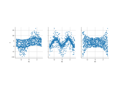
Create a polynomial chaos for the Ishigami function: a quick start guide to polynomial chaos
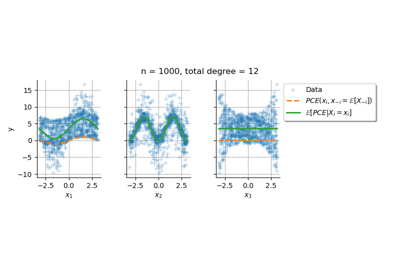
Conditional expectation of a polynomial chaos expansion
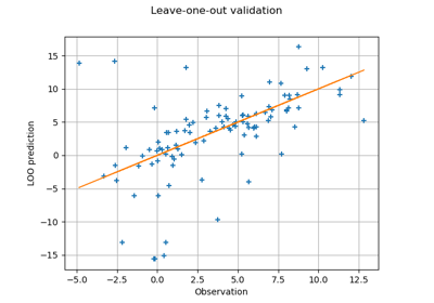
Compute leave-one-out error of a polynomial chaos expansion
 OpenTURNS

