Note
Go to the end to download the full example code.
Create a polynomial chaos for the Ishigami function: a quick start guide to polynomial chaos
In this example, we create a polynomial chaos for the
Ishigami function.
We create a sparse polynomial with maximum total degree equal to 8
using the FunctionalChaosAlgorithm class.
Define the model
from openturns.usecases import ishigami_function
import openturns as ot
import openturns.viewer as otv
import math

ot.Log.Show(ot.Log.NONE)
ot.RandomGenerator.SetSeed(0)
We load the Ishigami model :
im = ishigami_function.IshigamiModel()
The IshigamiModel data class contains the input distribution  in im.inputDistribution and the Ishigami function in im.model.
We also have access to the input variable names with
in im.inputDistribution and the Ishigami function in im.model.
We also have access to the input variable names with
input_names = im.inputDistribution.getDescription()
Draw the function
Create a training sample
sampleSize = 1000
inputSample = im.inputDistribution.getSample(sampleSize)
outputSample = im.model(inputSample)
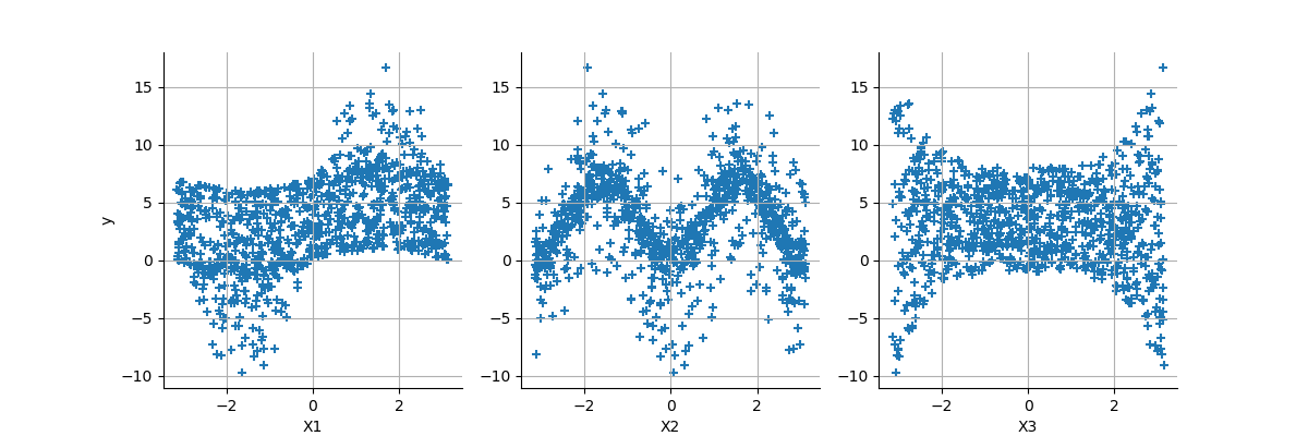
Display relationships between the output and the inputs
grid = ot.VisualTest.DrawPairsXY(inputSample, outputSample)
view = otv.View(grid, figure_kw={"figsize": (12.0, 4.0)})
graph = ot.HistogramFactory().build(outputSample).drawPDF()
view = otv.View(graph)
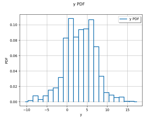
We see that the distribution of the output has two modes.
Create the polynomial chaos model
Create a training sample
sampleSize = 100
inputTrain = im.inputDistribution.getSample(sampleSize)
outputTrain = im.model(inputTrain)
Create the chaos.
We could use only the input and output training samples: in this case, the distribution of the input sample is computed by selecting the distribution that has the best fit.
chaosalgo = ot.FunctionalChaosAlgorithm(inputTrain, outputTrain)
Since the input distribution is known in our particular case, we instead create the multivariate basis from the distribution. We define the orthogonal basis used to expand the function. We see that each input has the uniform distribution, which corresponds to the Legendre polynomials.
multivariateBasis = ot.OrthogonalProductPolynomialFactory([im.X1, im.X2, im.X3])
multivariateBasis
Then we create the sparse polynomial chaos expansion using regression and the LARS selection model method.
selectionAlgorithm = ot.LeastSquaresMetaModelSelectionFactory()
projectionStrategy = ot.LeastSquaresStrategy(selectionAlgorithm)
totalDegree = 8
enumerateFunction = multivariateBasis.getEnumerateFunction()
basisSize = enumerateFunction.getBasisSizeFromTotalDegree(totalDegree)
adaptiveStrategy = ot.FixedStrategy(multivariateBasis, basisSize)
chaosAlgo = ot.FunctionalChaosAlgorithm(
    inputTrain, outputTrain, im.inputDistribution, adaptiveStrategy, projectionStrategy
)
The coefficients of the polynomial expansion can then be estimated
using the run() method.
chaosAlgo.run()
The getResult() method returns the
result.
chaosResult = chaosAlgo.getResult()
The polynomial chaos result provides a pretty-print.
chaosResult
Get the metamodel.
metamodel = chaosResult.getMetaModel()
In order to validate the metamodel, we generate a test sample.
n_valid = 1000
inputTest = im.inputDistribution.getSample(n_valid)
outputTest = im.model(inputTest)
metamodelPredictions = metamodel(inputTest)
val = ot.MetaModelValidation(outputTest, metamodelPredictions)
r2Score = val.computeR2Score()[0]
r2Score
0.9994752470145457
The  is very close to 1: the metamodel is accurate.
graph = val.drawValidation()
graph.setTitle("R2=%.2f%%" % (r2Score * 100))
view = otv.View(graph)
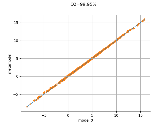
The metamodel has a good predictivity, since the points are almost on the first diagonal.
Compute mean and variance
The mean and variance of a polynomial chaos expansion are computed
using the coefficients of the expansion.
This can be done using FunctionalChaosRandomVector.
randomVector = ot.FunctionalChaosRandomVector(chaosResult)
mean = randomVector.getMean()
print("Mean=", mean)
covarianceMatrix = randomVector.getCovariance()
print("Covariance=", covarianceMatrix)
outputDimension = outputTrain.getDimension()
stdDev = ot.Point(outputDimension)
for i in range(outputDimension):
    stdDev[i] = math.sqrt(covarianceMatrix[i, i])
print("Standard deviation=", stdDev)
Mean= [3.51725]
Covariance= [[ 13.7368 ]]
Standard deviation= [3.70631]
Compute and print Sobol’ indices
By default, printing the object will print the Sobol’ indices
and the multi-indices ordered by decreasing part of variance.
If a multi-index has a part of variance which is lower
than some threshold, it is not printed.
This threshold can be customized using the
FunctionalChaosSobolIndices-VariancePartThreshold key of the
ResourceMap.
chaosSI = ot.FunctionalChaosSobolIndices(chaosResult)
chaosSI
We notice that a coefficient with marginal degree equal to 6 has a significant impact on the output variance. Hence, we cannot get a satisfactory polynomial chaos with total degree less that 6.
Draw Sobol’ indices.
dim_input = im.inputDistribution.getDimension()
first_order = [chaosSI.getSobolIndex(i) for i in range(dim_input)]
total_order = [chaosSI.getSobolTotalIndex(i) for i in range(dim_input)]
input_names = im.model.getInputDescription()
graph = ot.SobolIndicesAlgorithm.DrawSobolIndices(input_names, first_order, total_order)
view = otv.View(graph)
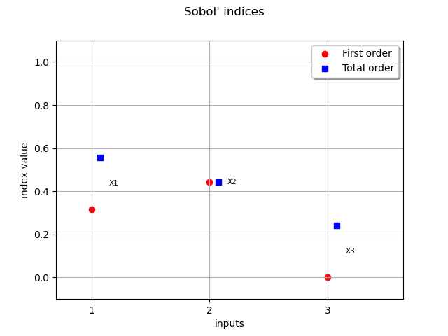
The variable which has the largest impact on the output is, taking
interactions into account,  .
We see that has interactions with other variables, since the first
order indice is less than the total order indice.
At first order,
.
We see that has interactions with other variables, since the first
order indice is less than the total order indice.
At first order,  has no interaction with other variables since its
first order indice is close to zero.
has no interaction with other variables since its
first order indice is close to zero.
Computing the accuracy
The interesting point with the Ishigami function is that the exact Sobol’ indices are known. We can use that property in order to compute the absolute error on the Sobol’ indices for the polynomial chaos.
To make the comparisons simpler, we gather the results into a list.
S_exact = [im.S1, im.S2, im.S3]
ST_exact = [im.ST1, im.ST2, im.ST3]
Then we perform a loop over the input dimension and compute the absolute error on the Sobol’ indices.
for i in range(im.dim):
    absoluteErrorS = abs(first_order[i] - S_exact[i])
    absoluteErrorST = abs(total_order[i] - ST_exact[i])
    print(
        "X%d, Abs.Err. on S=%.1e, Abs.Err. on ST=%.1e"
        % (i + 1, absoluteErrorS, absoluteErrorST)
    )
X1, Abs.Err. on S=1.3e-03, Abs.Err. on ST=4.4e-04
X2, Abs.Err. on S=4.1e-04, Abs.Err. on ST=4.8e-04
X3, Abs.Err. on S=4.8e-07, Abs.Err. on ST=1.7e-03
We see that the indices are correctly estimated with a low accuracy even if we have used only 100 function evaluations. This shows the good performance of the polynomial chaos in this case.
We can compute the part of the variance of the output explained by each multi-index.
partOfVariance = chaosSI.getPartOfVariance()
chaosResult = chaosSI.getFunctionalChaosResult()
coefficients = chaosResult.getCoefficients()
orthogonalBasis = chaosResult.getOrthogonalBasis()
enumerateFunction = orthogonalBasis.getEnumerateFunction()
indices = chaosResult.getIndices()
basisSize = indices.getSize()
print("Index, global index, multi-index, coefficient, part of variance")
for i in range(basisSize):
    globalIndex = indices[i]
    multiIndex = enumerateFunction(globalIndex)
    if partOfVariance[i] > 1.0e-3:
        print(
            "%d, %d, %s, %.4f, %.4f"
            % (i, globalIndex, multiIndex, coefficients[i, 0], partOfVariance[i])
        )
Index, global index, multi-index, coefficient, part of variance
1, 1, [1,0,0], 1.6229, 0.1917
3, 7, [0,2,0], -0.5899, 0.0253
4, 10, [3,0,0], -1.2886, 0.1209
5, 15, [1,0,2], 1.3625, 0.1351
6, 30, [0,4,0], -1.9398, 0.2739
8, 35, [5,0,0], 0.1883, 0.0026
9, 40, [3,0,2], -1.0812, 0.0851
10, 49, [1,0,4], 0.4107, 0.0123
11, 77, [0,6,0], 1.3586, 0.1344
13, 89, [5,0,2], 0.1603, 0.0019
14, 98, [3,0,4], -0.3199, 0.0075
19, 156, [0,8,0], -0.3556, 0.0092
view.show()