The Ishigami function
The Ishigami function of Ishigami & Homma (1990) is recurrent test case for sensitivity analysis methods and uncertainty.
Let  and
and  (see Crestaux et al. (2007) and Marrel et al. (2009)). We consider the function

for any ![X_1,X_2,X_3\in[-\pi,\pi]](data:image/svg+xml;base64,PD94bWwgdmVyc2lvbj0nMS4wJyBlbmNvZGluZz0nVVRGLTgnPz4KPCEtLSBUaGlzIGZpbGUgd2FzIGdlbmVyYXRlZCBieSBkdmlzdmdtIDMuNC4yIC0tPgo8c3ZnIHZlcnNpb249JzEuMScgeG1sbnM9J2h0dHA6Ly93d3cudzMub3JnLzIwMDAvc3ZnJyB4bWxuczp4bGluaz0naHR0cDovL3d3dy53My5vcmcvMTk5OS94bGluaycgd2lkdGg9JzEwMy42MjcyNTlwdCcgaGVpZ2h0PScxMS45NTUxNjhwdCcgdmlld0JveD0nMCAtOC45NjYzNzYgMTAzLjYyNzI1OSAxMS45NTUxNjgnPgo8ZGVmcz4KPHBhdGggaWQ9J2czLTkxJyBkPSdNMi45ODg3OTIgMi45ODg3OTJWMi41NDY0NTFIMS44MjkxNDFWLTguNTI0MDM1SDIuOTg4NzkyVi04Ljk2NjM3NkgxLjM4NjhWMi45ODg3OTJIMi45ODg3OTJaJy8+CjxwYXRoIGlkPSdnMy05MycgZD0nTTEuODUzMDUxLTguOTY2Mzc2SC4yNTEwNTlWLTguNTI0MDM1SDEuNDEwNzFWMi41NDY0NTFILjI1MTA1OVYyLjk4ODc5MkgxLjg1MzA1MVYtOC45NjYzNzZaJy8+CjxwYXRoIGlkPSdnMC0wJyBkPSdNNy44Nzg0NTYtMi43NDk2ODlDOC4wODE2OTQtMi43NDk2ODkgOC4yOTY4ODctMi43NDk2ODkgOC4yOTY4ODctMi45ODg3OTJTOC4wODE2OTQtMy4yMjc4OTUgNy44Nzg0NTYtMy4yMjc4OTVIMS40MTA3MUMxLjIwNzQ3Mi0zLjIyNzg5NSAuOTkyMjc5LTMuMjI3ODk1IC45OTIyNzktMi45ODg3OTJTMS4yMDc0NzItMi43NDk2ODkgMS40MTA3MS0yLjc0OTY4OUg3Ljg3ODQ1NlonLz4KPHBhdGggaWQ9J2cwLTUwJyBkPSdNNi41NTE0MzItMi43NDk2ODlDNi43NTQ2Ny0yLjc0OTY4OSA2Ljk2OTg2My0yLjc0OTY4OSA2Ljk2OTg2My0yLjk4ODc5MlM2Ljc1NDY3LTMuMjI3ODk1IDYuNTUxNDMyLTMuMjI3ODk1SDEuNDgyNDQxQzEuNjI1OTAzLTQuODI5ODg4IDMuMDAwNzQ3LTUuOTc3NTg0IDQuNjg2NDI2LTUuOTc3NTg0SDYuNTUxNDMyQzYuNzU0NjctNS45Nzc1ODQgNi45Njk4NjMtNS45Nzc1ODQgNi45Njk4NjMtNi4yMTY2ODdTNi43NTQ2Ny02LjQ1NTc5MSA2LjU1MTQzMi02LjQ1NTc5MUg0LjY2MjUxNkMyLjYxODE4Mi02LjQ1NTc5MSAuOTkyMjc5LTQuOTAxNjE5IC45OTIyNzktMi45ODg3OTJTMi42MTgxODIgLjQ3ODIwNyA0LjY2MjUxNiAuNDc4MjA3SDYuNTUxNDMyQzYuNzU0NjcgLjQ3ODIwNyA2Ljk2OTg2MyAuNDc4MjA3IDYuOTY5ODYzIC4yMzkxMDNTNi43NTQ2NyAwIDYuNTUxNDMyIDBINC42ODY0MjZDMy4wMDA3NDcgMCAxLjYyNTkwMy0xLjE0NzY5NiAxLjQ4MjQ0MS0yLjc0OTY4OUg2LjU1MTQzMlonLz4KPHBhdGggaWQ9J2cyLTQ5JyBkPSdNMi41MDI2MTUtNS4wNzY5NjFDMi41MDI2MTUtNS4yOTIxNTQgMi40ODY2NzUtNS4zMDAxMjUgMi4yNzE0ODItNS4zMDAxMjVDMS45NDQ3MDctNC45ODEzMiAxLjUyMjI5MS00Ljc5MDAzNyAuNzY1MTMxLTQuNzkwMDM3Vi00LjUyNzAyNEMuOTgwMzI0LTQuNTI3MDI0IDEuNDEwNzEtNC41MjcwMjQgMS44NzI5NzYtNC43NDIyMTdWLS42NTM1NDlDMS44NzI5NzYtLjM1ODY1NSAxLjg0OTA2Ni0uMjYzMDE0IDEuMDkxOTA1LS4yNjMwMTRILjgxMjk1MVYwQzEuMTM5NzI2LS4wMjM5MSAxLjgyNTE1Ni0uMDIzOTEgMi4xODM4MTEtLjAyMzkxUzMuMjM1ODY2LS4wMjM5MSAzLjU2MjY0IDBWLS4yNjMwMTRIMy4yODM2ODZDMi41MjY1MjYtLjI2MzAxNCAyLjUwMjYxNS0uMzU4NjU1IDIuNTAyNjE1LS42NTM1NDlWLTUuMDc2OTYxWicvPgo8cGF0aCBpZD0nZzItNTAnIGQ9J00yLjI0NzU3Mi0xLjYyNTkwM0MyLjM3NTA5My0xLjc0NTQ1NSAyLjcwOTgzOC0yLjAwODQ2OCAyLjgzNzM2LTIuMTIwMDVDMy4zMzE1MDctMi41NzQzNDYgMy44MDE3NDMtMy4wMTI3MDIgMy44MDE3NDMtMy43Mzc5ODNDMy44MDE3NDMtNC42ODY0MjYgMy4wMDQ3MzItNS4zMDAxMjUgMi4wMDg0NjgtNS4zMDAxMjVDMS4wNTIwNTUtNS4zMDAxMjUgLjQyMjQxNi00LjU3NDg0NCAuNDIyNDE2LTMuODY1NTA0Qy40MjI0MTYtMy40NzQ5NjkgLjczMzI1LTMuNDE5MTc4IC44NDQ4MzItMy40MTkxNzhDMS4wMTIyMDQtMy40MTkxNzggMS4yNTkyNzgtMy41Mzg3MyAxLjI1OTI3OC0zLjg0MTU5NEMxLjI1OTI3OC00LjI1NjA0IC44NjA3NzItNC4yNTYwNCAuNzY1MTMxLTQuMjU2MDRDLjk5NjI2NC00LjgzNzg1OCAxLjUzMDI2Mi01LjAzNzExMSAxLjkyMDc5Ny01LjAzNzExMUMyLjY2MjAxNy01LjAzNzExMSAzLjA0NDU4My00LjQwNzQ3MiAzLjA0NDU4My0zLjczNzk4M0MzLjA0NDU4My0yLjkwOTA5MSAyLjQ2Mjc2NS0yLjMwMzM2MiAxLjUyMjI5MS0xLjMzODk3OUwuNTE4MDU3LS4zMDI4NjRDLjQyMjQxNi0uMjE1MTkzIC40MjI0MTYtLjE5OTI1MyAuNDIyNDE2IDBIMy41NzA2MUwzLjgwMTc0My0xLjQyNjY1SDMuNTU0NjdDMy41MzA3Ni0xLjI2NzI0OCAzLjQ2Njk5OS0uODY4NzQyIDMuMzcxMzU3LS43MTczMUMzLjMyMzUzNy0uNjUzNTQ5IDIuNzE3ODA4LS42NTM1NDkgMi41OTAyODYtLjY1MzU0OUgxLjE3MTYwNkwyLjI0NzU3Mi0xLjYyNTkwM1onLz4KPHBhdGggaWQ9J2cyLTUxJyBkPSdNMi4wMTY0MzgtMi42NjIwMTdDMi42NDYwNzctMi42NjIwMTcgMy4wNDQ1ODMtMi4xOTk3NTEgMy4wNDQ1ODMtMS4zNjI4ODlDMy4wNDQ1ODMtLjM2NjYyNSAyLjQ3ODcwNS0uMDcxNzMxIDIuMDU2Mjg5LS4wNzE3MzFDMS42MTc5MzMtLjA3MTczMSAxLjAyMDE3NC0uMjMxMTMzIC43NDEyMi0uNjUzNTQ5QzEuMDI4MTQ0LS42NTM1NDkgMS4yMjczOTctLjgzNjg2MiAxLjIyNzM5Ny0xLjA5OTg3NUMxLjIyNzM5Ny0xLjM1NDkxOSAxLjA0NDA4NS0xLjUzODIzMiAuNzg5MDQxLTEuNTM4MjMyQy41NzM4NDgtMS41MzgyMzIgLjM1MDY4NS0xLjQwMjc0IC4zNTA2ODUtMS4wODM5MzVDLjM1MDY4NS0uMzI2Nzc1IDEuMTYzNjM2IC4xNjczNzIgMi4wNzIyMjkgLjE2NzM3MkMzLjEzMjI1NCAuMTY3MzcyIDMuODczNDc0LS41NjU4NzggMy44NzM0NzQtMS4zNjI4ODlDMy44NzM0NzQtMi4wMjQ0MDggMy4zNDc0NDctMi42MzAxMzcgMi41MzQ0OTYtMi44MDU0NzlDMy4xNjQxMzQtMy4wMjg2NDMgMy42MzQzNzEtMy41NzA2MSAzLjYzNDM3MS00LjIwODIxOVMyLjkxNzA2MS01LjMwMDEyNSAyLjA4ODE2OS01LjMwMDEyNUMxLjIzNTM2Ny01LjMwMDEyNSAuNTg5Nzg4LTQuODM3ODU4IC41ODk3ODgtNC4yMzIxM0MuNTg5Nzg4LTMuOTM3MjM1IC43ODkwNDEtMy44MDk3MTQgLjk5NjI2NC0zLjgwOTcxNEMxLjI0MzMzNy0zLjgwOTcxNCAxLjQwMjc0LTMuOTg1MDU2IDEuNDAyNzQtNC4yMTYxODlDMS40MDI3NC00LjUxMTA4MyAxLjE0NzY5Ni00LjYyMjY2NSAuOTcyMzU0LTQuNjMwNjM1QzEuMzA3MDk4LTUuMDY4OTkxIDEuOTIwNzk3LTUuMDkyOTAyIDIuMDY0MjU5LTUuMDkyOTAyQzIuMjcxNDgyLTUuMDkyOTAyIDIuODc3MjEtNS4wMjkxNDEgMi44NzcyMS00LjIwODIxOUMyLjg3NzIxLTMuNjUwMzExIDIuNjQ2MDc3LTMuMzE1NTY3IDIuNTM0NDk2LTMuMTg4MDQ1QzIuMjk1MzkyLTIuOTQwOTcxIDIuMTEyMDgtMi45MjUwMzEgMS42MjU5MDMtMi44OTMxNTFDMS40NzQ0NzEtMi44ODUxODEgMS40MTA3MS0yLjg3NzIxIDEuNDEwNzEtMi43NzM1OTlDMS40MTA3MS0yLjY2MjAxNyAxLjQ4MjQ0MS0yLjY2MjAxNyAxLjYxNzkzMy0yLjY2MjAxN0gyLjAxNjQzOFonLz4KPHBhdGggaWQ9J2cxLTI1JyBkPSdNMy4wOTYzODktNC41MDcwOThINC40NDczMjNDNC4xMjQ1MzMtMy4xNjgxMiAzLjkyMTI5NS0yLjI5NTM5MiAzLjkyMTI5NS0xLjMzODk3OUMzLjkyMTI5NS0xLjE3MTYwNiAzLjkyMTI5NSAuMTE5NTUyIDQuNDExNDU3IC4xMTk1NTJDNC42NjI1MTYgLjExOTU1MiA0Ljg3NzcwOS0uMTA3NTk3IDQuODc3NzA5LS4zMTA4MzRDNC44Nzc3MDktLjM3MDYxIDQuODc3NzA5LS4zOTQ1MjEgNC43OTQwMjItLjU3Mzg0OEM0LjQ3MTIzMy0xLjM5ODc1NSA0LjQ3MTIzMy0yLjQyNjg5OSA0LjQ3MTIzMy0yLjUxMDU4NUM0LjQ3MTIzMy0yLjU4MjMxNiA0LjQ3MTIzMy0zLjQzMTEzMyA0LjcyMjI5MS00LjUwNzA5OEg2LjA2MTI3QzYuMjE2Njg3LTQuNTA3MDk4IDYuNjExMjA4LTQuNTA3MDk4IDYuNjExMjA4LTQuODg5NjY0QzYuNjExMjA4LTUuMTUyNjc3IDYuMzg0MDYtNS4xNTI2NzcgNi4xNjg4NjctNS4xNTI2NzdIMi4yMzU2MTZDMS45NjA2NDgtNS4xNTI2NzcgMS41NTQxNzItNS4xNTI2NzcgMS4wMDQyMzQtNC41NjY4NzRDLjY5MzQtNC4yMjAxNzQgLjMxMDgzNC0zLjU4NjU1IC4zMTA4MzQtMy41MTQ4MTlTLjM3MDYxLTMuNDE5MTc4IC40NDIzNDEtMy40MTkxNzhDLjUyNjAyNy0zLjQxOTE3OCAuNTM3OTgzLTMuNDU1MDQ0IC41OTc3NTgtMy41MjY3NzVDMS4yMTk0MjctNC41MDcwOTggMS44NDEwOTYtNC41MDcwOTggMi4xMzk5NzUtNC41MDcwOThIMi44MjE0MkMyLjU1ODQwNi0zLjYxMDQ2MSAyLjI1OTUyNy0yLjU3MDM2MSAxLjI3OTIwMy0uNDc4MjA3QzEuMTgzNTYyLS4yODY5MjQgMS4xODM1NjItLjI2MzAxNCAxLjE4MzU2Mi0uMTkxMjgzQzEuMTgzNTYyIC4wNTk3NzYgMS4zOTg3NTUgLjExOTU1MiAxLjUwNjM1MSAuMTE5NTUyQzEuODUzMDUxIC4xMTk1NTIgMS45NDg2OTItLjE5MTI4MyAyLjA5MjE1NC0uNjkzNEMyLjI4MzQzNy0xLjMwMzExMyAyLjI4MzQzNy0xLjMyNzAyNCAyLjQwMjk4OS0xLjgwNTIzTDMuMDk2Mzg5LTQuNTA3MDk4WicvPgo8cGF0aCBpZD0nZzEtNTknIGQ9J00yLjMzMTI1OCAuMDQ3ODIxQzIuMzMxMjU4LS42NDU1NzkgMi4xMDQxMS0xLjE1OTY1MSAxLjYxMzk0OC0xLjE1OTY1MUMxLjIzMTM4Mi0xLjE1OTY1MSAxLjA0MDEtLjg0ODgxNyAxLjA0MDEtLjU4NTgwM1MxLjIxOTQyNyAwIDEuNjI1OTAzIDBDMS43ODEzMiAwIDEuOTEyODI3LS4wNDc4MjEgMi4wMjA0MjMtLjE1NTQxN0MyLjA0NDMzNC0uMTc5MzI4IDIuMDU2Mjg5LS4xNzkzMjggMi4wNjgyNDQtLjE3OTMyOEMyLjA5MjE1NC0uMTc5MzI4IDIuMDkyMTU0LS4wMTE5NTUgMi4wOTIxNTQgLjA0NzgyMUMyLjA5MjE1NCAuNDQyMzQxIDIuMDIwNDIzIDEuMjE5NDI3IDEuMzI3MDI0IDEuOTk2NTEzQzEuMTk1NTE3IDIuMTM5OTc1IDEuMTk1NTE3IDIuMTYzODg1IDEuMTk1NTE3IDIuMTg3Nzk2QzEuMTk1NTE3IDIuMjQ3NTcyIDEuMjU1MjkzIDIuMzA3MzQ3IDEuMzE1MDY4IDIuMzA3MzQ3QzEuNDEwNzEgMi4zMDczNDcgMi4zMzEyNTggMS40MjI2NjUgMi4zMzEyNTggLjA0NzgyMVonLz4KPHBhdGggaWQ9J2cxLTg4JyBkPSdNNS42Nzg3MDUtNC44NTM3OThMNC41NTQ5MTktNy40NzE5OEM0LjcxMDMzNi03Ljc1ODkwNCA1LjA2ODk5MS03LjgwNjcyNSA1LjIxMjQ1My03LjgxODY4QzUuMjg0MTg0LTcuODE4NjggNS40MTU2OTEtNy44MzA2MzUgNS40MTU2OTEtOC4wMzM4NzNDNS40MTU2OTEtOC4xNjUzOCA1LjMwODA5NS04LjE2NTM4IDUuMjM2MzY0LTguMTY1MzhDNS4wMzMxMjYtOC4xNjUzOCA0Ljc5NDAyMi04LjE0MTQ2OSA0LjU5MDc4NS04LjE0MTQ2OUgzLjg5NzM4NUMzLjE2ODEyLTguMTQxNDY5IDIuNjQyMDkyLTguMTY1MzggMi42MzAxMzctOC4xNjUzOEMyLjUzNDQ5Ni04LjE2NTM4IDIuNDE0OTQ0LTguMTY1MzggMi40MTQ5NDQtNy45MzgyMzJDMi40MTQ5NDQtNy44MTg2OCAyLjUyMjU0LTcuODE4NjggMi42Nzc5NTgtNy44MTg2OEMzLjM3MTM1Ny03LjgxODY4IDMuNDE5MTc4LTcuNjk5MTI4IDMuNTM4NzMtNy40MTIyMDRMNC45NjEzOTUtNC4wODg2NjdMMi4zNjcxMjMtMS4zMTUwNjhDMS45MzY3MzctLjg0ODgxNyAxLjQyMjY2NS0uMzk0NTIxIC41Mzc5ODMtLjM0NjdDLjM5NDUyMS0uMzM0NzQ1IC4yOTg4NzktLjMzNDc0NSAuMjk4ODc5LS4xMTk1NTJDLjI5ODg3OS0uMDgzNjg2IC4zMTA4MzQgMCAuNDQyMzQxIDBDLjYwOTcxNCAwIC43ODkwNDEtLjAyMzkxIC45NTY0MTMtLjAyMzkxSDEuNTE4MzA2QzEuOTAwODcyLS4wMjM5MSAyLjMxOTMwMyAwIDIuNjg5OTEzIDBDMi43NzM1OTkgMCAyLjkxNzA2MSAwIDIuOTE3MDYxLS4yMTUxOTNDMi45MTcwNjEtLjMzNDc0NSAyLjgzMzM3NS0uMzQ2NyAyLjc2MTY0NC0uMzQ2N0MyLjUyMjU0LS4zNzA2MSAyLjM2NzEyMy0uNTAyMTE3IDIuMzY3MTIzLS42OTM0QzIuMzY3MTIzLS44OTY2MzggMi41MTA1ODUtMS4wNDAxIDIuODU3Mjg1LTEuMzk4NzU1TDMuOTIxMjk1LTIuNTU4NDA2QzQuMTg0MzA5LTIuODMzMzc1IDQuODE3OTMzLTMuNTI2Nzc1IDUuMDgwOTQ2LTMuNzg5Nzg4TDYuMzM2MjM5LS44NDg4MTdDNi4zNDgxOTQtLjgyNDkwNyA2LjM5NjAxNS0uNzA1MzU1IDYuMzk2MDE1LS42OTM0QzYuMzk2MDE1LS41ODU4MDMgNi4xMzMwMDEtLjM3MDYxIDUuNzUwNDM2LS4zNDY3QzUuNjc4NzA1LS4zNDY3IDUuNTQ3MTk4LS4zMzQ3NDUgNS41NDcxOTgtLjExOTU1MkM1LjU0NzE5OCAwIDUuNjY2NzUgMCA1LjcyNjUyNiAwQzUuOTI5NzYzIDAgNi4xNjg4NjctLjAyMzkxIDYuMzcyMTA1LS4wMjM5MUg3LjY4NzE3M0M3LjkwMjM2Ni0uMDIzOTEgOC4xMjk1MTQgMCA4LjMzMjc1MiAwQzguNDE2NDM4IDAgOC41NDc5NDUgMCA4LjU0Nzk0NS0uMjI3MTQ4QzguNTQ3OTQ1LS4zNDY3IDguNDI4Mzk0LS4zNDY3IDguMzIwNzk3LS4zNDY3QzcuNjAzNDg3LS4zNTg2NTUgNy41Nzk1NzctLjQxODQzMSA3LjM3NjMzOS0uODYwNzcyTDUuNzk4MjU3LTQuNTY2ODc0TDcuMzE2NTYzLTYuMTkyNzc3QzcuNDM2MTE1LTYuMzEyMzI5IDcuNzExMDgzLTYuNjExMjA4IDcuODE4NjgtNi43MzA3NkM4LjMzMjc1Mi03LjI2ODc0MiA4LjgxMDk1OS03Ljc1ODkwNCA5Ljc3OTMyOC03LjgxODY4QzkuODk4ODc5LTcuODMwNjM1IDEwLjAxODQzMS03LjgzMDYzNSAxMC4wMTg0MzEtOC4wMzM4NzNDMTAuMDE4NDMxLTguMTY1MzggOS45MTA4MzQtOC4xNjUzOCA5Ljg2MzAxNC04LjE2NTM4QzkuNjk1NjQxLTguMTY1MzggOS41MTYzMTQtOC4xNDE0NjkgOS4zNDg5NDEtOC4xNDE0NjlIOC43OTkwMDRDOC40MTY0MzgtOC4xNDE0NjkgNy45OTgwMDctOC4xNjUzOCA3LjYyNzM5Ny04LjE2NTM4QzcuNTQzNzExLTguMTY1MzggNy40MDAyNDktOC4xNjUzOCA3LjQwMDI0OS03Ljk1MDE4N0M3LjQwMDI0OS03LjgzMDYzNSA3LjQ4MzkzNS03LjgxODY4IDcuNTU1NjY2LTcuODE4NjhDNy43NDY5NDktNy43OTQ3NyA3Ljk1MDE4Ny03LjY5OTEyOCA3Ljk1MDE4Ny03LjQ3MTk4TDcuOTM4MjMyLTcuNDQ4MDdDNy45MjYyNzYtNy4zNjQzODQgNy45MDIzNjYtNy4yNDQ4MzIgNy43NzA4NTktNy4xMDEzN0w1LjY3ODcwNS00Ljg1Mzc5OFonLz4KPC9kZWZzPgo8ZyBpZD0ncGFnZTEnPgo8dXNlIHg9JzAnIHk9JzAnIHhsaW5rOmhyZWY9JyNnMS04OCcvPgo8dXNlIHg9JzkuNzE1MjI3JyB5PScxLjc5MzI2MycgeGxpbms6aHJlZj0nI2cyLTQ5Jy8+Cjx1c2UgeD0nMTQuNDQ3NTQyJyB5PScwJyB4bGluazpocmVmPScjZzEtNTknLz4KPHVzZSB4PScxOS42OTE3MDEnIHk9JzAnIHhsaW5rOmhyZWY9JyNnMS04OCcvPgo8dXNlIHg9JzI5LjQwNjkyOCcgeT0nMS43OTMyNjMnIHhsaW5rOmhyZWY9JyNnMi01MCcvPgo8dXNlIHg9JzM0LjEzOTI0MycgeT0nMCcgeGxpbms6aHJlZj0nI2cxLTU5Jy8+Cjx1c2UgeD0nMzkuMzgzNDAyJyB5PScwJyB4bGluazpocmVmPScjZzEtODgnLz4KPHVzZSB4PSc0OS4wOTg2MjknIHk9JzEuNzkzMjYzJyB4bGluazpocmVmPScjZzItNTEnLz4KPHVzZSB4PSc1Ny4xNTE3NzQnIHk9JzAnIHhsaW5rOmhyZWY9JyNnMC01MCcvPgo8dXNlIHg9JzY4LjQ0Mjc0MicgeT0nMCcgeGxpbms6aHJlZj0nI2czLTkxJy8+Cjx1c2UgeD0nNzEuNjk0NDAzJyB5PScwJyB4bGluazpocmVmPScjZzAtMCcvPgo8dXNlIHg9JzgwLjk5MjknIHk9JzAnIHhsaW5rOmhyZWY9JyNnMS0yNScvPgo8dXNlIHg9Jzg4LjA2MjE3JyB5PScwJyB4bGluazpocmVmPScjZzEtNTknLz4KPHVzZSB4PSc5My4zMDYzMjgnIHk9JzAnIHhsaW5rOmhyZWY9JyNnMS0yNScvPgo8dXNlIHg9JzEwMC4zNzU1OTgnIHk9JzAnIHhsaW5rOmhyZWY9JyNnMy05MycvPgo8L2c+Cjwvc3ZnPgo8IS0tIERFUFRIPTQgLS0+) We assume that the random variables
We assume that the random variables  are independent and have the uniform marginal distribution in the interval from
  to
to  :
:

Analysis
The expectation and the variance of  are
are

and

The Sobol’ decomposition variances are

and  .
.
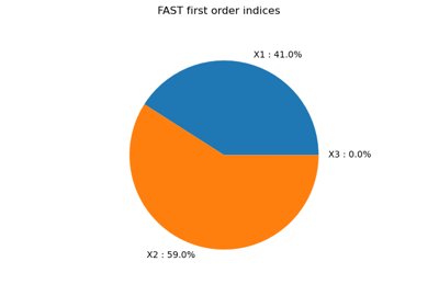
This leads to the following first order Sobol’ indices:

and the following total order indices:

The third variable  has no effect at first order (because
  it is multiplied
by
it is multiplied
by  ), but has a total effet because of the interactions with
  .
On the other hand, the second variable
.
On the other hand, the second variable  has no interactions which implies
that the first order indice is equal to the total order indice for this input variable.
has no interactions which implies
that the first order indice is equal to the total order indice for this input variable.
References
Ishigami, T., & Homma, T. (1990, December). An importance quantification technique in uncertainty analysis for computer models. In Uncertainty Modeling and Analysis, 1990. Proceedings., First International Symposium on (pp. 398-403). IEEE.
Sobol’, I. M., & Levitan, Y. L. (1999). On the use of variance reducing multipliers in Monte Carlo computations of a global sensitivity index. Computer Physics Communications, 117(1), 52-61.
Crestaux, T., Martinez, J.-M., Le Maitre, O., & Lafitte, O. (2007). Polynomial chaos expansion for uncertainties quantification and sensitivity analysis. SAMO 2007, http://samo2007.chem.elte.hu/lectures/Crestaux.pdf.
Load the use case
We can load this model from the use cases module as follows :
>>> from openturns.usecases import ishigami_function
>>> # Load the Ishigami use case
>>> im = ishigami_function.IshigamiModel()
API documentation
- class IshigamiModel
Data class for the Ishigami model.
- Attributes:
- dimThe dimension of the problem
dim = 3
- afloat
Constant: a = 7.0
- bfloat
Constant: b = 0.1
- X1
Uniform First marginal, ot.Uniform(-np.pi, np.pi)
- X2
Uniform Second marginal, ot.Uniform(-np.pi, np.pi)
- X3
Uniform Third marginal, ot.Uniform(-np.pi, np.pi)
- inputDistribution
JointDistribution The joint distribution of the input parameters.
- ishigami
SymbolicFunction The Ishigami model with a, b as variables.
- model
ParametricFunction The Ishigami model with the a=7.0 and b=0.1 parameters fixed.
- expectationfloat
Expectation of the output variable.
- variancefloat
Variance of the output variable.
- S1float
First order Sobol index number 1
- S2float
First order Sobol index number 2
- S3float
First order Sobol index number 3
- S12float
Second order Sobol index for marginals 1 and 2.
- S13float
Second order Sobol index for marginals 1 and 3.
- S23float
Second order Sobol index for marginals 2 and 3.
- S123float
- ST1float
Total order Sobol index number 1.
- ST2float
Total order Sobol index number 2.
- ST3float
Total order Sobol index number 3.
Examples
>>> from openturns.usecases import ishigami_function
>>> # Load the Ishigami model
>>> im = ishigami_function.IshigamiModel()
Examples based on this use case

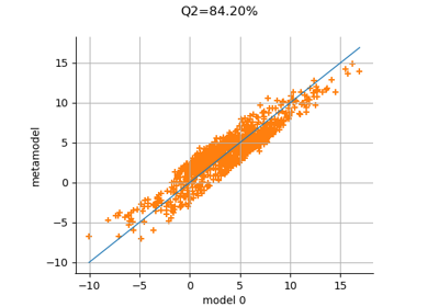
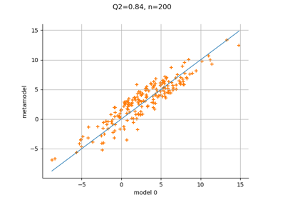
Create a polynomial chaos for the Ishigami function: a quick start guide to polynomial chaos
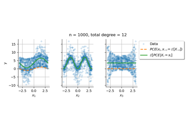
Conditional expectation of a polynomial chaos expansion
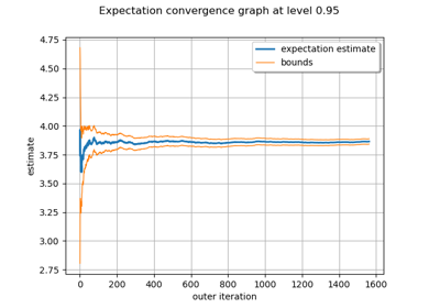
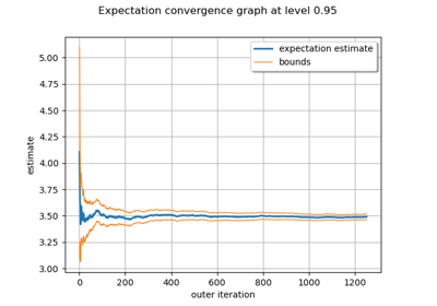
Evaluate the mean of a random vector by simulations
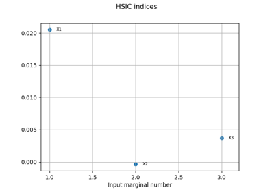
Sobol’ sensitivity indices using rank-based algorithm

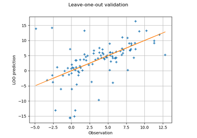
Compute leave-one-out error of a polynomial chaos expansion