FunctionalChaosAlgorithm
- class FunctionalChaosAlgorithm(*args)
Functional chaos algorithm.
Refer to Functional Chaos Expansion, Least squares polynomial response surface.
- Available constructors:
FunctionalChaosAlgorithm(inputSample, outputSample)
FunctionalChaosAlgorithm(inputSample, outputSample, distribution)
FunctionalChaosAlgorithm(inputSample, outputSample, distribution, adaptiveStrategy)
FunctionalChaosAlgorithm(inputSample, outputSample, distribution, adaptiveStrategy, projectionStrategy)
FunctionalChaosAlgorithm(inputSample, weights, outputSample, distribution, adaptiveStrategy)
FunctionalChaosAlgorithm(inputSample, weights, outputSample, distribution, adaptiveStrategy, projectionStrategy)
- Parameters:
- inputSample: 2-d sequence of float
Sample of the input random vectors with size
 and dimension
  .
.- outputSample: 2-d sequence of float
Sample of the output random vectors with size
and dimension  .
.- distribution
Distribution Distribution of the random vector
 of dimension .
When the distribution is unspecified, the
of dimension .
When the distribution is unspecified, the
BuildDistribution()static method is evaluated on the inputSample.- adaptiveStrategy
AdaptiveStrategy Strategy of selection of the different terms of the multivariate basis.
- projectionStrategy
ProjectionStrategy Strategy of evaluation of the coefficients

- weightssequence of float
Weights
 associated to the output
sample, where is the sample size.
Default values are
associated to the output
sample, where is the sample size.
Default values are  for
for  .
.
Methods
BuildDistribution(inputSample)Recover the distribution, with metamodel performance in mind.
Get the adaptive strategy.
Accessor to the object's name.
Accessor to the joint probability density function of the physical input vector.
Accessor to the input sample.
Get the maximum residual.
getName()Accessor to the object's name.
Accessor to the output sample.
Get the projection strategy.
Get the results of the metamodel computation.
Return the weights of the input sample.
hasName()Test if the object is named.
run()Compute the metamodel.
setDistribution(distribution)Accessor to the joint probability density function of the physical input vector.
setMaximumResidual(residual)Set the maximum residual.
setName(name)Accessor to the object's name.
setProjectionStrategy(projectionStrategy)Set the projection strategy.
See also
Notes
This class creates a functional chaos expansion or polynomial chaos expansion (PCE) based on an input and output sample of the physical model. More details on this type of surrogate models are presented in Functional Chaos Expansion. Once the expansion is computed, the
FunctionalChaosRandomVectorclass provides methods to get the mean and variance of the PCE. Moreover, theFunctionalChaosSobolIndicesprovides Sobol’ indices of the PCE.Default settings for the adaptive strategy
When the adaptiveStrategy is unspecified, the FunctionalChaosAlgorithm-QNorm parameter of the
ResourceMapis used. If this parameter is equal to 1, then theLinearEnumerateFunctionclass is used. Otherwise, theHyperbolicAnisotropicEnumerateFunctionclass is used. If the FunctionalChaosAlgorithm-BasisSize key of theResourceMapis nonzero, then this parameter sets the basis size. Otherwise, the FunctionalChaosAlgorithm-MaximumTotalDegree key of theResourceMapis used to compute the basis size using the getBasisSizeFromTotalDegree method of the orthogonal basis (with a maximum of terms due to the sample size).
Finally, the FixedStrategyclass is used.Default settings for the projection strategy
When the projectionStrategy is unspecified, the FunctionalChaosAlgorithm-Sparse key of the
ResourceMapis used. If it is false, then theLeastSquaresStrategyclass is used, which produces a full PCE, without model selection. Otherwise, aLARSPCE is created, i.e. a sparse PCE is computed using model selection. In this case, the FunctionalChaosAlgorithm-FittingAlgorithm key of theResourceMapis used.If this key is equal to ‘CorrectedLeaveOneOut’, then the
CorrectedLeaveOneOutcriteria is used.If this key is equal to ‘KFold’, then the
KFoldcriteria is used.Otherwise, an exception is produced.
Examples
Create the model:
>>> import openturns as ot
>>> ot.RandomGenerator.SetSeed(0)
>>> inputDimension = 1
>>> model = ot.SymbolicFunction(['x'], ['x * sin(x)'])
>>> distribution = ot.JointDistribution([ot.Uniform()] * inputDimension)
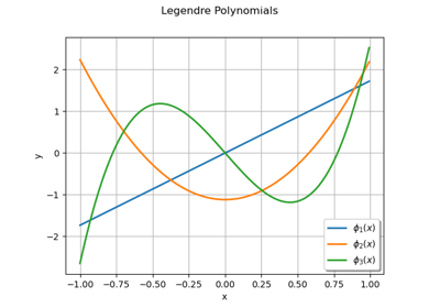
Build the multivariate orthonormal basis:
>>> polyColl = [0.0] * inputDimension
>>> for i in range(distribution.getDimension()):
...     polyColl[i] = ot.StandardDistributionPolynomialFactory(distribution.getMarginal(i))
>>> enumerateFunction = ot.LinearEnumerateFunction(inputDimension)
>>> productBasis = ot.OrthogonalProductPolynomialFactory(polyColl, enumerateFunction)
Define the strategy to truncate the multivariate orthonormal basis: We choose all the polynomials of degree lower or equal to 4.
>>> degree = 4
>>> indexMax = enumerateFunction.getBasisSizeFromTotalDegree(degree)
>>> print(indexMax)
5
We keep all the polynomials of degree lower or equal to 4 (which corresponds to the 5 first ones):
>>> adaptiveStrategy = ot.FixedStrategy(productBasis, indexMax)
Define the evaluation strategy of the coefficients:
>>> samplingSize = 50
>>> experiment = ot.MonteCarloExperiment(distribution, samplingSize)
>>> inputSample = experiment.generate()
>>> outputSample = model(inputSample)
>>> projectionStrategy = ot.LeastSquaresStrategy()
Create the chaos algorithm:
>>> algo = ot.FunctionalChaosAlgorithm(
...     inputSample, outputSample, distribution, adaptiveStrategy, projectionStrategy
... )
>>> algo.run()
Get the result:
>>> functionalChaosResult = algo.getResult()
>>> # print(functionalChaosResult)  # Pretty-print
>>> metamodel = functionalChaosResult.getMetaModel()
Test it:
>>> X = [0.5]
>>> print(model(X))
[0.239713]
>>> print(metamodel(X))
[0.239514]
There are several methods to define the algorithm: default settings are used when the information is not provided by the user. The simplest is to set only the input and output samples. In this case, the distribution and its parameters are estimated from the inputSample using the
BuildDistributionclass. See the Fit a distribution from an input sample example for more details on this topic.>>> algo = ot.FunctionalChaosAlgorithm(inputSample, outputSample)
In many cases, the distribution is known and it is best to use this information when we have it.
>>> algo = ot.FunctionalChaosAlgorithm(inputSample, outputSample, distribution)
A more involved method is to define the method to set the orthogonal basis of functions or polynomials. We use the
OrthogonalProductPolynomialFactoryclass to define the orthogonal basis of polynomials. Then we use theFixedStrategyto define the maximum number of candidate polynomials to consider in the expansion, up to the total degree equal to 10.>>> enumerateFunction = ot.LinearEnumerateFunction(inputDimension) >>> maximumTotalDegree = 10 >>> totalSize = enumerateFunction.getBasisSizeFromTotalDegree(maximumTotalDegree) >>> polynomialsList = [] >>> for i in range(inputDimension): ... marginalDistribution = distribution.getMarginal(i) ... marginalPolynomial = ot.StandardDistributionPolynomialFactory(marginalDistribution) ... polynomialsList.append(marginalPolynomial) >>> basis = ot.OrthogonalProductPolynomialFactory(polynomialsList, enumerateFunction) >>> adaptiveStrategy = ot.FixedStrategy(basis, totalSize) >>> algo = ot.FunctionalChaosAlgorithm( ... inputSample, outputSample, distribution, adaptiveStrategy ... )
The most involved method is to define the way to compute the coefficients, thanks to the
ProjectionStrategy. In the next example, we useLARSto create a sparse PCE.>>> selection = ot.LeastSquaresMetaModelSelectionFactory( ... ot.LARS(), ... ot.CorrectedLeaveOneOut() ... ) >>> projectionStrategy = ot.LeastSquaresStrategy(inputSample, outputSample, selection) >>> algo = ot.FunctionalChaosAlgorithm( ... inputSample, outputSample, distribution, adaptiveStrategy, projectionStrategy ... )
- __init__(*args)
- static BuildDistribution(inputSample)
Recover the distribution, with metamodel performance in mind.
For each marginal, find the best 1-d continuous parametric model else fallback to the use of a nonparametric one.
The selection is done as follow:
We start with a list of all parametric models (all factories)
For each model, we estimate its parameters if feasible.
We check then if model is valid, ie if its Kolmogorov score exceeds a threshold fixed in the MetaModelAlgorithm-PValueThreshold ResourceMap key. Default value is 5%
We sort all valid models and return the one with the optimal criterion.
For the last step, the criterion might be BIC, AIC or AICC. The specification of the criterion is done through the MetaModelAlgorithm-ModelSelectionCriterion ResourceMap key. Default value is fixed to BIC. Note that if there is no valid candidate, we estimate a non-parametric model (
KernelSmoothingorHistogram). The MetaModelAlgorithm-NonParametricModel ResourceMap key allows selecting the preferred one. Default value is HistogramOne each marginal is estimated, we use the Spearman independence test on each component pair to decide whether an independent copula. In case of non independence, we rely on a
NormalCopula.- Parameters:
- sample
Sample Input sample.
- sample
- Returns:
- distribution
Distribution Input distribution.
- distribution
- getAdaptiveStrategy()
Get the adaptive strategy.
- Returns:
- adaptiveStrategy
AdaptiveStrategy Strategy of selection of the different terms of the multivariate basis.
- adaptiveStrategy
- getClassName()
Accessor to the object’s name.
- Returns:
- class_namestr
The object class name (object.__class__.__name__).
- getDistribution()
Accessor to the joint probability density function of the physical input vector.
- Returns:
- distribution
Distribution Joint probability density function of the physical input vector.
- distribution
- getInputSample()
Accessor to the input sample.
- Returns:
- inputSample
Sample Input sample of a model evaluated apart.
- inputSample
- getMaximumResidual()
Get the maximum residual.
- Returns:
- residualfloat
Residual value needed in the projection strategy.
Default value is
 .
.
- getName()
Accessor to the object’s name.
- Returns:
- namestr
The name of the object.
- getOutputSample()
Accessor to the output sample.
- Returns:
- outputSample
Sample Output sample of a model evaluated apart.
- outputSample
- getProjectionStrategy()
Get the projection strategy.
- Returns:
- strategy
ProjectionStrategy Projection strategy.
- strategy
Notes
The projection strategy selects the different terms of the multivariate basis to define the subset K.
- getResult()
Get the results of the metamodel computation.
- Returns:
- result
FunctionalChaosResult Result structure, created by the method
run().
- result
- getWeights()
Return the weights of the input sample.
- Returns:
- weightssequence of float
The weights of the points in the input sample.
- hasName()
Test if the object is named.
- Returns:
- hasNamebool
True if the name is not empty.
- run()
Compute the metamodel.
Notes
Evaluates the metamodel and stores all the results in a result structure.
- setDistribution(distribution)
Accessor to the joint probability density function of the physical input vector.
- Parameters:
- distribution
Distribution Joint probability density function of the physical input vector.
- distribution
- setMaximumResidual(residual)
Set the maximum residual.
- Parameters:
- residualfloat
Residual value needed in the projection strategy.
Default value is
.
- setName(name)
Accessor to the object’s name.
- Parameters:
- namestr
The name of the object.
- setProjectionStrategy(projectionStrategy)
Set the projection strategy.
- Parameters:
- projectionStrategy
ProjectionStrategy Strategy to estimate the coefficients
.
- projectionStrategy
Examples using the class


Create a full or sparse polynomial chaos expansion
Create a polynomial chaos metamodel by integration on the cantilever beam

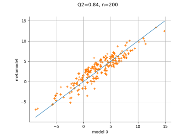
Create a polynomial chaos metamodel from a data set
Create a polynomial chaos for the Ishigami function: a quick start guide to polynomial chaos
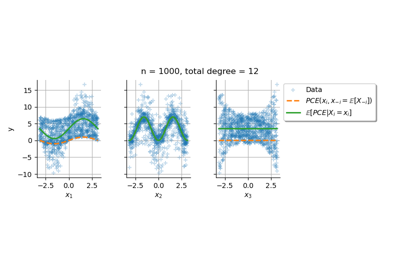
Conditional expectation of a polynomial chaos expansion
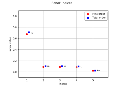
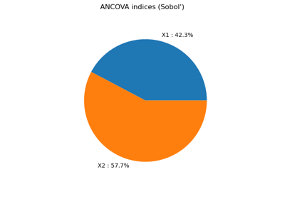
Example of sensitivity analyses on the wing weight model
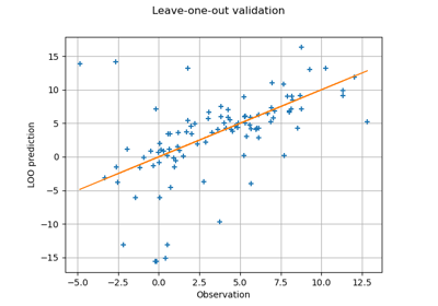
Compute leave-one-out error of a polynomial chaos expansion