Compute Sobol’ indices confidence intervals

In this example we will estimate confidence intervals for chaos Sobol’ indices by bootstrap. Unlike estimation by sampling where the confidence intervals are obtained from the asymptotic distributions, there is currently no known analytical method to compute Sobol’ confidence intervals, so we can fallback to bootstrap.

Bootstraping the polynomial chaos is presented in [marelli2018] as “full bootstraping” and referred to as bootstrap-PCE or bPCE. Full bPCE can be CPU time consuming in some cases, e.g. when the dimension of the input random vector is large or when the training sample size is large. In the fast bPCE method, the sparse polynomial basis identified by the LARS algorithm is computed only once. Then bootstrapping is applied to the regression step on the sparse basis. Using fast bPCE is not straightforward, so we use full bPCE in the current example.

To do this, we must simultaneously bootstrap in the input and output samples, so that the input/output mapping is preserved. In the example below, we show how to use the BootstrapExperiment class for this purpose.

This involves the following steps:

• Generate an initial input/output design of experiment.

• Compute a fixed number of bootstrap samples from the original design.

• For each input/output boostrap samples, compute Sobol’ indices by functional chaos.

• Compute quantiles of these Sobol’ indices realizations to get the confidence intervals.

import openturns as ot
from openturns.usecases import cantilever_beam
import openturns.viewer as otv

Load the cantilever beam use-case. We want to use the independent distribution to get meaningful Sobol’ indices.

beam = cantilever_beam.CantileverBeam()
g = beam.model
distribution = beam.independentDistribution
dim_input = distribution.getDimension()

Create the tensorized polynomial basis, with the default linear enumeration function.

marginals = [distribution.getMarginal(i) for i in range(dim_input)]
basis = ot.OrthogonalProductPolynomialFactory(marginals)

Generate a learning sample with MC simulation (or retrieve the design from experimental data).

ot.RandomGenerator.SetSeed(0)
N = 35  # size of the experimental design
X = distribution.getSample(N)
Y = g(X)

def computeSparseLeastSquaresChaos(X, Y, basis, total_degree, distribution):
    """
    Create a sparse polynomial chaos with least squares.

    * Uses the enumeration rule from basis.
    * Uses LeastSquaresStrategy to compute the coefficients from
    linear least squares.
    * Uses LeastSquaresMetaModelSelectionFactory to select the polynomials
    in the basis using least angle regression stepwise (LARS)
    * Utilise LeastSquaresStrategy pour calculer les
    coefficients par moindres carrés.
    * Uses FixedStrategy to keep all coefficients that LARS has selected,
    up to the given maximum total degree.

    Parameters
    ----------
    X : Sample(n)
        The input training design of experiments with n points
    Y : Sample(n)
        The input training design of experiments with n points
    basis : Basis
        The multivariate orthogonal polynomial basis
    total_degree : int
        The maximum total polynomial degree
    distribution : Distribution
        The distribution of the input random vector

    Returns
    -------
    result : FunctionalChaosResult
        The polynomial chaos result
    """
    selectionAlgorithm = ot.LeastSquaresMetaModelSelectionFactory()
    projectionStrategy = ot.LeastSquaresStrategy(selectionAlgorithm)
    enum_func = basis.getEnumerateFunction()
    P = enum_func.getBasisSizeFromTotalDegree(total_degree)
    adaptiveStrategy = ot.FixedStrategy(basis, P)
    algo = ot.FunctionalChaosAlgorithm(
        X, Y, distribution, adaptiveStrategy, projectionStrategy
    )
    algo.run()
    result = algo.getResult()
    return result

Build the chaos metamodel on the design of experiment.

total_degree = 3
result = computeSparseLeastSquaresChaos(X, Y, basis, total_degree, distribution)
metamodel = result.getMetaModel()

Generate a validation sample independent of the training sample.

n_valid = 1000
X_test = distribution.getSample(n_valid)
Y_test = g(X_test)

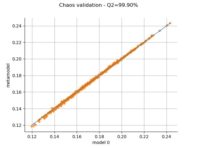
The MetaModelValidation class allows one to validate the metamodel on a test sample. Plot the observed versus the predicted outputs.

val = ot.MetaModelValidation(X_test, Y_test, metamodel)
graph = val.drawValidation()
Q2 = val.computePredictivityFactor()[0]
graph.setTitle(f"Chaos validation - Q2={Q2*100.0:.2f}%")
_ = otv.View(graph)

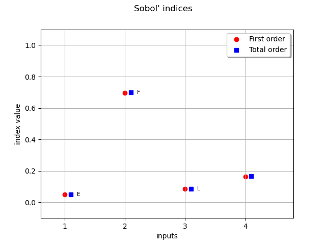
Retrieve Sobol’ sensitivity measures associated to the polynomial chaos decomposition of the model.

chaosSI = ot.FunctionalChaosSobolIndices(result)
fo_indices = [chaosSI.getSobolIndex(i) for i in range(dim_input)]
to_indices = [chaosSI.getSobolTotalIndex(i) for i in range(dim_input)]
input_names = g.getInputDescription()
graph = ot.SobolIndicesAlgorithm.DrawSobolIndices(input_names, fo_indices, to_indices)
_ = otv.View(graph)

We define the multiBootstrap function in order to simultaneously bootstrap in the input and output samples, so that the input/output mapping is preserved. We use the GenerateSelection method of the BootstrapExperiment class.

def multiBootstrap(*data):
    """
    Bootstrap multiple samples at once.

    Parameters
    ----------
    data : sequence of Sample
        Multiple samples to bootstrap.

    Returns
    -------
    data_boot : sequence of Sample
        The bootstrap samples.
    """
    assert len(data) > 0, "empty list"
    size = data[0].getSize()
    selection = ot.BootstrapExperiment.GenerateSelection(size, size)
    return [Z[selection] for Z in data]

Generate input/output bootstrap samples from the initial design.

X_boot, Y_boot = multiBootstrap(X, Y)
print(X_boot[:5])
print(Y_boot[:5])

    [ E             F             L             I             ]
0 : [   7.09376e+10 305.568         2.55637       1.34556e-07 ]
1 : [   6.5963e+10  228.332         2.57804       1.53991e-07 ]
2 : [   6.60008e+10 325.25          2.5146        1.45825e-07 ]
3 : [   6.52443e+10 320.71          2.54539       1.40993e-07 ]
4 : [   6.86026e+10 282.187         2.59881       1.42475e-07 ]
    [ y0       ]
0 : [ 0.178271 ]
1 : [ 0.128386 ]
2 : [ 0.179111 ]
3 : [ 0.191651 ]
4 : [ 0.168912 ]

def computeChaosSensitivity(X, Y, basis, total_degree, distribution):
    """
    Compute the first and total order Sobol' indices from a polynomial chaos.

    Parameters
    ----------
    X, Y : Sample
        Input/Output design
    basis : Basis
        Tensorized basis
    total_degree : int
        Maximal total degree
    distribution : Distribution
        Input distribution

    Returns
    -------
    first_order, total_order: list of float
        The first and total order indices.
    """
    dim_input = X.getDimension()
    result = computeSparseLeastSquaresChaos(X, Y, basis, total_degree, distribution)
    chaosSI = ot.FunctionalChaosSobolIndices(result)
    first_order = [chaosSI.getSobolIndex(i) for i in range(dim_input)]
    total_order = [chaosSI.getSobolTotalIndex(i) for i in range(dim_input)]
    return first_order, total_order

def computeBootstrapChaosSobolIndices(
    X, Y, basis, total_degree, distribution, bootstrap_size
):
    """
    Computes a bootstrap sample of first and total order indices from polynomial chaos.

    Parameters
    ----------
    X, Y : Sample
        Input/Output design
    basis : Basis
        Tensorized basis
    total_degree : int
        Maximal total degree
    distribution : Distribution
        Input distribution
    bootstrap_size : interval
        The bootstrap sample size
    """
    dim_input = X.getDimension()
    fo_sample = ot.Sample(0, dim_input)
    to_sample = ot.Sample(0, dim_input)
    unit_eps = ot.Interval([1e-9] * dim_input, [1 - 1e-9] * dim_input)
    for i in range(bootstrap_size):
        X_boot, Y_boot = multiBootstrap(X, Y)
        first_order, total_order = computeChaosSensitivity(
            X_boot, Y_boot, basis, total_degree, distribution
        )
        if unit_eps.contains(first_order) and unit_eps.contains(total_order):
            fo_sample.add(first_order)
            to_sample.add(total_order)
    return fo_sample, to_sample

Compute sample of Sobol’ indices by boostrap.

bootstrap_size = 500
fo_sample, to_sample = computeBootstrapChaosSobolIndices(
    X, Y, basis, total_degree, distribution, bootstrap_size
)

def computeSobolIndicesConfidenceInterval(fo_sample, to_sample, alpha=0.95):
    """
    From a sample of first or total order indices,
    compute a bilateral confidence interval of level alpha.

    Estimates the distribution of the first and total order Sobol' indices
    from a bootstrap estimation.
    Then computes a bilateral confidence interval for each marginal.

    Parameters
    ----------
    fo_sample: ot.Sample(n, dim_input)
        The first order indices
    to_sample: ot.Sample(n, dim_input)
        The total order indices
    alpha : float
        The confidence level

    Returns
    -------
    fo_interval : ot.Interval
        The confidence interval of first order Sobol' indices
    to_interval : ot.Interval
        The confidence interval of total order Sobol' indices
    """
    dim_input = fo_sample.getDimension()
    fo_lb = [0] * dim_input
    fo_ub = [0] * dim_input
    to_lb = [0] * dim_input
    to_ub = [0] * dim_input
    for i in range(dim_input):
        fo_i = fo_sample[:, i]
        to_i = to_sample[:, i]
        beta = (1.0 - alpha) / 2
        fo_lb[i] = fo_i.computeQuantile(beta)[0]
        fo_ub[i] = fo_i.computeQuantile(1.0 - beta)[0]
        to_lb[i] = to_i.computeQuantile(beta)[0]
        to_ub[i] = to_i.computeQuantile(1.0 - beta)[0]

    # Create intervals
    fo_interval = ot.Interval(fo_lb, fo_ub)
    to_interval = ot.Interval(to_lb, to_ub)
    return fo_interval, to_interval

Compute confidence intervals from the indices samples.

fo_interval, to_interval = computeSobolIndicesConfidenceInterval(fo_sample, to_sample)

def computeAndDrawSobolIndices(
    N, basis, total_degree, distribution, bootstrap_size=500, alpha=0.95
):
    """
    Compute and draw Sobol' indices from a polynomial chaos based on a
    given sample size.
    Compute confidence intervals at level alpha from bootstrap.
    """
    X = distribution.getSample(N)
    Y = g(X)
    fo_sample, to_sample = computeBootstrapChaosSobolIndices(
        X, Y, basis, total_degree, distribution, bootstrap_size
    )

    fo_interval, to_interval = computeSobolIndicesConfidenceInterval(
        fo_sample, to_sample, alpha
    )

    graph = ot.SobolIndicesAlgorithm.DrawSobolIndices(
        input_names,
        fo_sample.computeMean(),
        to_sample.computeMean(),
        fo_interval,
        to_interval,
    )
    graph.setTitle(f"Sobol' indices - N={N}")
    graph.setIntegerXTick(True)
    return graph

Plot the boostrap Sobol’ indices mean and the confidence intervals. The confidence length will shrink if we increase the initial sample size.

sphinx_gallery_thumbnail_number = 3

graph = computeAndDrawSobolIndices(30, basis, total_degree, distribution)
_ = otv.View(graph)

otv.View.ShowAll()

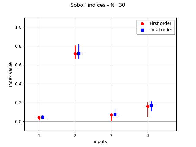
We see that the variable F has the highest sensitivity indices and that confidence intervals do not change this conclusion. The confidence intervals of the sensitivity indices of the variables L and I are similar so that we cannot say which of L or I is more significant than the other: both variables have similar sensitivity indices. The least sensitive variable is E, but the confidence intervals do not cross the X axis. Hence, there is no evidence that the Sobol’ indices of E are zero.