Note
Go to the end to download the full example code.
Create a sparse chaos by integration
The goal of this example is to show how to create a sparse polynomial chaos
expansion (PCE) when we estimate its coefficients by integration. We show
how to use the CleaningStrategy class.
Polynomial chaos expansion
Let  be a function
where
be a function
where  is the domain of
  .
We consider
.
We consider  a random vector which
probability density function is denoted by
a random vector which
probability density function is denoted by  .
We assume that
.
We assume that  has a finite second order moment.
Let
has a finite second order moment.
Let  be an iso-probabilistic transformation such that
  follows a distribution uniquely defined by all its moments.
Let
follows a distribution uniquely defined by all its moments.
Let  be the function defined by:

The polynomial chaos decomposition of with respect to the measure of
 is (see [blatman2009] page 73) :

where  is a multi-index,
  is the
coefficient,
is the
coefficient,  is a multivariate polynomial.
Truncated expansion
In practice, we cannot consider an infinite series and must truncate the decomposition at a given order. Only a selection of coefficients must be kept. This leads to a subset of all possible multi-indices. In the remainder of this text, we call this selection the multi-index set.
Several multi-index sets can be considered. A simple method is to truncate
the polynomial up to a given maximum total degree  .
Let
.
Let  be the multi-index set defined by

where

is the 1-norm of the multi-index  .
Therefore, the truncated polynomial chaos expansion is:
.
Therefore, the truncated polynomial chaos expansion is:

In order to ensure a low error, we may choose a large value of the
parameter  . This, however, leads to a large number of
coefficients
. This, however, leads to a large number of
coefficients  to
estimate. More precisely, the number of coefficients to estimate
is (see [blatman2009] page 73) :
to
estimate. More precisely, the number of coefficients to estimate
is (see [blatman2009] page 73) :

where  is the factorial number of
  .
.
Low-rank polynomial chaos expansion
For any  , let
, let
 be the rank of the multi-index, that is,
the number of non-zero components:
be the rank of the multi-index, that is,
the number of non-zero components:

where  is the indicator function.
The multi-index set of maximum total degree
and maximum rank
is the indicator function.
The multi-index set of maximum total degree
and maximum rank  is ([blatman2009] page 74):

Therefore, the rank-j polynomial chaos expansion is:

The rank is now a hyperparameter of the model: [blatman2009] suggests
to use  . An example of low-rank PCE for the G-Sobol’
function is given in [blatman2009] page 75.
. An example of low-rank PCE for the G-Sobol’
function is given in [blatman2009] page 75.
Note. It is currently not possible to create a low-rank PCE.
Model selection
If  is large, many coefficients
may be poorly estimated, which may reduce the quality of the metamodel. We may
want to select a subset of the coefficients which best predict the output.
In other words, we may compute a subset:
is large, many coefficients
may be poorly estimated, which may reduce the quality of the metamodel. We may
want to select a subset of the coefficients which best predict the output.
In other words, we may compute a subset:

such that ([blatman2009] page 86) :

An enumeration rule is a function from the set of integers  to
the corresponding set of multi-indices . More
precisely, let
to
the corresponding set of multi-indices . More
precisely, let  be the
function such that :
be the
function such that :

for any  .
Let
.
Let  be a parameter representing the number of
coefficients considered in the selection. Given an enumeration rule for
the multi-indices , at most
be a parameter representing the number of
coefficients considered in the selection. Given an enumeration rule for
the multi-indices , at most  multi-indices
will be considered. Let
multi-indices
will be considered. Let  be the corresponding multi-index set :

Let  be a parameter representing the minimum relative
value of a significant coefficient
be a parameter representing the minimum relative
value of a significant coefficient  .
The
.
The CleaningStrategy uses the following criterion to select the coefficients :

where  is the significance factor, which by default is
 . This rule selects only the coefficients which
are significantly different from zero.
. This rule selects only the coefficients which
are significantly different from zero.
Sparsity index
The sparsity index of a multi-index set is the ratio of the cardinality of
the multi-index set to the cardinality of the multi-index set of the
equivalent multi-index with maximum total degree. For a given multi-index
set  , let
, let  be the maximum 1-norm of multi-indices
in the set :
be the maximum 1-norm of multi-indices
in the set :

The index of sparsity of is ([blatman2009] eq. 4.42 page 86) :

Note. The index of sparsity as defined by [blatman2009] is close to zero when the model is very sparse. The following complementary indicator is close to 1 when the model is very sparse:

import openturns as ot
import openturns.viewer as otv
from openturns.usecases import ishigami_function
import itertools
The following function takes a polynomial chaos result as input and prints a given maximum number of coefficients of this polynomial. It can take into account a threshold, so that we can avoid to print coefficients which are very close to zero.
def printCoefficientsTable(
    polynomialChaosResult, maximum_number_of_printed_coefficients=10, threshold=0.0
):
    """
    Print the coefficients of the polynomial chaos.

    Parameters
    ----------
    polynomialChaosResult : ot.FunctionalChaosResult
        The polynomial chaos expansion.
    maximum_number_of_printed_coefficients : int
        The maximum number of printed coefficients.
    threshold : float, strictly positive
        If a coefficient has an absolute value strictly greater than the
        threshold, it is printed.
    """
    basis = polynomialChaosResult.getOrthogonalBasis()
    coefficients = polynomialChaosResult.getCoefficients()
    enumerate_function = basis.getEnumerateFunction()
    indices = polynomialChaosResult.getIndices()
    nbcoeffs = indices.getSize()
    print("Total number of coefficients : ", nbcoeffs)
    print("# Indice, Multi-indice, Degree : Value")
    print_index = 0
    for k in range(nbcoeffs):
        multiindex = enumerate_function(indices[k])
        degree = sum(multiindex)
        c = coefficients[k][0]
        if abs(c) > threshold:
            print("#%d, %s (%s) : %s" % (k, multiindex, degree, c))
            print_index += 1
        if print_index > maximum_number_of_printed_coefficients:
            break
    return
The next function computes the polynomial chaos  score using simple validation
on a test sample generated by Monte-Carlo sampling. The actual computation
is performed by the
score using simple validation
on a test sample generated by Monte-Carlo sampling. The actual computation
is performed by the MetaModelValidation class.
def compute_polynomial_chaos_R2(
    polynomialchaos_result, g_function, input_distribution, n_valid=1000
):
    """
    Compute the R2 score of the polynomial chaos.


    Parameters
    ----------
    polynomialChaosResult : ot.FunctionalChaosResult
        The polynomial chaos expansion.
    g_function : ot.Function
        The function.
    input_distribution : ot.Distribution
        The input distribution.
    n_valid : int
        The number of simulations to compute the R2 score.

    Returns
    -------
    r2Score : float
        The R2 score
    """
    ot.RandomGenerator.SetSeed(1976)
    metamodel = polynomialchaos_result.getMetaModel()
    inputTest = input_distribution.getSample(n_valid)
    outputTest = g_function(inputTest)
    metamodelPredictions = metamodel(inputTest)
    val = ot.MetaModelValidation(outputTest, metamodelPredictions)
    r2Score = val.computeR2Score()[0]
    return r2Score
The following function creates a validation plot using the
drawValidation() method
of the MetaModelValidation class.
def draw_polynomial_chaos_validation(
    polynomialchaos_result, g_function, input_distribution, n_valid=1000
):
    """
    Validate the polynomial chaos.

    Create the validation plot.


    Parameters
    ----------
    polynomialChaosResult : ot.FunctionalChaosResult
        The polynomial chaos expansion.
    g_function : ot.Function
        The function.
    input_distribution : ot.Distribution
        The input distribution.
    n_valid : int
        The number of simulations to compute the R2 score.

    Returns
    -------
    view : ot.View
        The plot.
    """
    metamodel = polynomialchaos_result.getMetaModel()
    inputTest = input_distribution.getSample(n_valid)
    outputTest = g_function(inputTest)
    metamodelPredictions = metamodel(inputTest)
    val = ot.MetaModelValidation(outputTest, metamodelPredictions)
    r2Score = val.computeR2Score()[0]
    graph = val.drawValidation()
    graph.setTitle("R2=%.2f%%" % (r2Score * 100))
    view = otv.View(graph, figure_kw={"figsize": (5.0, 4.0)})
    return view
We consider the Ishigami model.
Its three inputs are i.i.d. random variables that follow the uniform distribution on the
![[-\pi, \pi]](data:image/svg+xml;base64,PD94bWwgdmVyc2lvbj0nMS4wJyBlbmNvZGluZz0nVVRGLTgnPz4KPCEtLSBUaGlzIGZpbGUgd2FzIGdlbmVyYXRlZCBieSBkdmlzdmdtIDMuNC4yIC0tPgo8c3ZnIHZlcnNpb249JzEuMScgeG1sbnM9J2h0dHA6Ly93d3cudzMub3JnLzIwMDAvc3ZnJyB4bWxuczp4bGluaz0naHR0cDovL3d3dy53My5vcmcvMTk5OS94bGluaycgd2lkdGg9JzM1LjE4NDUxOHB0JyBoZWlnaHQ9JzExLjk1NTE2OHB0JyB2aWV3Qm94PScwIC04Ljk2NjM3NiAzNS4xODQ1MTggMTEuOTU1MTY4Jz4KPGRlZnM+CjxwYXRoIGlkPSdnMS0yNScgZD0nTTMuMDk2Mzg5LTQuNTA3MDk4SDQuNDQ3MzIzQzQuMTI0NTMzLTMuMTY4MTIgMy45MjEyOTUtMi4yOTUzOTIgMy45MjEyOTUtMS4zMzg5NzlDMy45MjEyOTUtMS4xNzE2MDYgMy45MjEyOTUgLjExOTU1MiA0LjQxMTQ1NyAuMTE5NTUyQzQuNjYyNTE2IC4xMTk1NTIgNC44Nzc3MDktLjEwNzU5NyA0Ljg3NzcwOS0uMzEwODM0QzQuODc3NzA5LS4zNzA2MSA0Ljg3NzcwOS0uMzk0NTIxIDQuNzk0MDIyLS41NzM4NDhDNC40NzEyMzMtMS4zOTg3NTUgNC40NzEyMzMtMi40MjY4OTkgNC40NzEyMzMtMi41MTA1ODVDNC40NzEyMzMtMi41ODIzMTYgNC40NzEyMzMtMy40MzExMzMgNC43MjIyOTEtNC41MDcwOThINi4wNjEyN0M2LjIxNjY4Ny00LjUwNzA5OCA2LjYxMTIwOC00LjUwNzA5OCA2LjYxMTIwOC00Ljg4OTY2NEM2LjYxMTIwOC01LjE1MjY3NyA2LjM4NDA2LTUuMTUyNjc3IDYuMTY4ODY3LTUuMTUyNjc3SDIuMjM1NjE2QzEuOTYwNjQ4LTUuMTUyNjc3IDEuNTU0MTcyLTUuMTUyNjc3IDEuMDA0MjM0LTQuNTY2ODc0Qy42OTM0LTQuMjIwMTc0IC4zMTA4MzQtMy41ODY1NSAuMzEwODM0LTMuNTE0ODE5Uy4zNzA2MS0zLjQxOTE3OCAuNDQyMzQxLTMuNDE5MTc4Qy41MjYwMjctMy40MTkxNzggLjUzNzk4My0zLjQ1NTA0NCAuNTk3NzU4LTMuNTI2Nzc1QzEuMjE5NDI3LTQuNTA3MDk4IDEuODQxMDk2LTQuNTA3MDk4IDIuMTM5OTc1LTQuNTA3MDk4SDIuODIxNDJDMi41NTg0MDYtMy42MTA0NjEgMi4yNTk1MjctMi41NzAzNjEgMS4yNzkyMDMtLjQ3ODIwN0MxLjE4MzU2Mi0uMjg2OTI0IDEuMTgzNTYyLS4yNjMwMTQgMS4xODM1NjItLjE5MTI4M0MxLjE4MzU2MiAuMDU5Nzc2IDEuMzk4NzU1IC4xMTk1NTIgMS41MDYzNTEgLjExOTU1MkMxLjg1MzA1MSAuMTE5NTUyIDEuOTQ4NjkyLS4xOTEyODMgMi4wOTIxNTQtLjY5MzRDMi4yODM0MzctMS4zMDMxMTMgMi4yODM0MzctMS4zMjcwMjQgMi40MDI5ODktMS44MDUyM0wzLjA5NjM4OS00LjUwNzA5OFonLz4KPHBhdGggaWQ9J2cxLTU5JyBkPSdNMi4zMzEyNTggLjA0NzgyMUMyLjMzMTI1OC0uNjQ1NTc5IDIuMTA0MTEtMS4xNTk2NTEgMS42MTM5NDgtMS4xNTk2NTFDMS4yMzEzODItMS4xNTk2NTEgMS4wNDAxLS44NDg4MTcgMS4wNDAxLS41ODU4MDNTMS4yMTk0MjcgMCAxLjYyNTkwMyAwQzEuNzgxMzIgMCAxLjkxMjgyNy0uMDQ3ODIxIDIuMDIwNDIzLS4xNTU0MTdDMi4wNDQzMzQtLjE3OTMyOCAyLjA1NjI4OS0uMTc5MzI4IDIuMDY4MjQ0LS4xNzkzMjhDMi4wOTIxNTQtLjE3OTMyOCAyLjA5MjE1NC0uMDExOTU1IDIuMDkyMTU0IC4wNDc4MjFDMi4wOTIxNTQgLjQ0MjM0MSAyLjAyMDQyMyAxLjIxOTQyNyAxLjMyNzAyNCAxLjk5NjUxM0MxLjE5NTUxNyAyLjEzOTk3NSAxLjE5NTUxNyAyLjE2Mzg4NSAxLjE5NTUxNyAyLjE4Nzc5NkMxLjE5NTUxNyAyLjI0NzU3MiAxLjI1NTI5MyAyLjMwNzM0NyAxLjMxNTA2OCAyLjMwNzM0N0MxLjQxMDcxIDIuMzA3MzQ3IDIuMzMxMjU4IDEuNDIyNjY1IDIuMzMxMjU4IC4wNDc4MjFaJy8+CjxwYXRoIGlkPSdnMC0wJyBkPSdNNy44Nzg0NTYtMi43NDk2ODlDOC4wODE2OTQtMi43NDk2ODkgOC4yOTY4ODctMi43NDk2ODkgOC4yOTY4ODctMi45ODg3OTJTOC4wODE2OTQtMy4yMjc4OTUgNy44Nzg0NTYtMy4yMjc4OTVIMS40MTA3MUMxLjIwNzQ3Mi0zLjIyNzg5NSAuOTkyMjc5LTMuMjI3ODk1IC45OTIyNzktMi45ODg3OTJTMS4yMDc0NzItMi43NDk2ODkgMS40MTA3MS0yLjc0OTY4OUg3Ljg3ODQ1NlonLz4KPHBhdGggaWQ9J2cyLTkxJyBkPSdNMi45ODg3OTIgMi45ODg3OTJWMi41NDY0NTFIMS44MjkxNDFWLTguNTI0MDM1SDIuOTg4NzkyVi04Ljk2NjM3NkgxLjM4NjhWMi45ODg3OTJIMi45ODg3OTJaJy8+CjxwYXRoIGlkPSdnMi05MycgZD0nTTEuODUzMDUxLTguOTY2Mzc2SC4yNTEwNTlWLTguNTI0MDM1SDEuNDEwNzFWMi41NDY0NTFILjI1MTA1OVYyLjk4ODc5MkgxLjg1MzA1MVYtOC45NjYzNzZaJy8+CjwvZGVmcz4KPGcgaWQ9J3BhZ2UxJz4KPHVzZSB4PScwJyB5PScwJyB4bGluazpocmVmPScjZzItOTEnLz4KPHVzZSB4PSczLjI1MTY2MScgeT0nMCcgeGxpbms6aHJlZj0nI2cwLTAnLz4KPHVzZSB4PScxMi41NTAxNTgnIHk9JzAnIHhsaW5rOmhyZWY9JyNnMS0yNScvPgo8dXNlIHg9JzE5LjYxOTQyOCcgeT0nMCcgeGxpbms6aHJlZj0nI2cxLTU5Jy8+Cjx1c2UgeD0nMjQuODYzNTg3JyB5PScwJyB4bGluazpocmVmPScjZzEtMjUnLz4KPHVzZSB4PSczMS45MzI4NTYnIHk9JzAnIHhsaW5rOmhyZWY9JyNnMi05MycvPgo8L2c+Cjwvc3ZnPgo8IS0tIERFUFRIPTQgLS0+) interval. This is an interesting example for our
purpose because it is highly non-linear, so that a high polynomial degree
will be required in order to produce a polynomial chaos expansion with
score sufficiently close to 1.
interval. This is an interesting example for our
purpose because it is highly non-linear, so that a high polynomial degree
will be required in order to produce a polynomial chaos expansion with
score sufficiently close to 1.
im = ishigami_function.IshigamiModel()

im.inputDistribution.setDescription(["`X_0`", "`X_1`", "`X_2`"])
im.model.setOutputDescription(["`Y`"])
print(im.inputDistribution)
JointDistribution(Uniform(a = -3.14159, b = 3.14159), Uniform(a = -3.14159, b = 3.14159), Uniform(a = -3.14159, b = 3.14159), IndependentCopula(dimension = 3))
Then we create the multivariate basis onto which the function is expanded.
By default, it is associated with the linear enumeration rule. Since our
marginals are uniform, the OrthogonalProductPolynomialFactory class
produces Legendre polynomials.
In order to create the multivariate basis of polynomials, we must specify the
number of functions in the basis. In this particular case, we compute that
number depending on the total degree.
The getMaximumDegreeStrataIndex() method
of the enumeration function computes the number of layers necessary to achieve
that total degree. Then the number of functions up to that layer is computed
with the getStrataCumulatedCardinal() method.
dimension = im.inputDistribution.getDimension()
multivariateBasis = ot.OrthogonalProductPolynomialFactory(
    [im.inputDistribution.getMarginal(i) for i in range(dimension)]
)

totalDegree = 5  # Polynomial degree
enumerate_function = multivariateBasis.getEnumerateFunction()
strataIndex = enumerate_function.getMaximumDegreeStrataIndex(totalDegree)
print("strataIndex = ", strataIndex)
number_of_terms_in_basis = enumerate_function.getStrataCumulatedCardinal(strataIndex)
print("number_of_terms_in_basis = ", number_of_terms_in_basis)
adaptiveStrategy = ot.FixedStrategy(multivariateBasis, number_of_terms_in_basis)
print(adaptiveStrategy)
strataIndex =  5
number_of_terms_in_basis =  56
class=FixedStrategy derived from class=AdaptiveStrategyImplementation maximumDimension=56
We compute the coefficients using a multivariate tensor product Gaussian
quadrature rule. Since the coefficients are computed in the standardized
space, we first use the getMeasure method of the multivariate basis in
order to get that standardized distribution. Then we use the
GaussProductExperiment class to create the quadrature,
using 6 nodes on each
of the dimensions.
standard_distribution = multivariateBasis.getMeasure()
print(standard_distribution)

marginal_number_of_nodes = 6
dim_input = im.model.getInputDimension()
marginalDegrees = [marginal_number_of_nodes] * dim_input
experiment = ot.GaussProductExperiment(im.inputDistribution, marginalDegrees)
X, W = experiment.generateWithWeights()
Y = im.model(X)
print("Sample size = ", X.getSize())
JointDistribution(Uniform(a = -1, b = 1), Uniform(a = -1, b = 1), Uniform(a = -1, b = 1), IndependentCopula(dimension = 3))
Sample size =  216
We see that 216 nodes are involved in this quadrature rule, which is the result
of  .
.
In the next cell, we compute the coefficients of the polynomial chaos expansion using integration.
projectionStrategy = ot.IntegrationStrategy()
chaosalgo = ot.FunctionalChaosAlgorithm(
    X, W, Y, im.inputDistribution, adaptiveStrategy, projectionStrategy
)
chaosalgo.run()
result = chaosalgo.getResult()
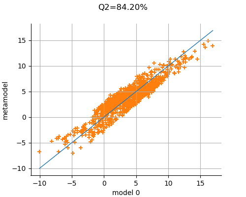
We now validate the metamodel by drawing the validation graph. We see that many points are close to the red test line, which indicates that the predictions of the polynomial chaos expansion are close to the output observations from the model.
view = draw_polynomial_chaos_validation(result, im.model, im.inputDistribution)
In order to have a closer look on the result, we use the printCoefficientsTable function in order to print the first 10 coefficients.
printCoefficientsTable(result)
Total number of coefficients :  56
# Indice, Multi-indice, Degree : Value
#0, [0,0,0] (0) : 3.5049783626206317
#1, [1,0,0] (1) : 1.6254291279668378
#2, [0,1,0] (1) : 9.189697613987136e-16
#3, [0,0,1] (1) : -1.7737547541862853e-16
#4, [2,0,0] (2) : -2.7590776885411117e-15
#5, [1,1,0] (2) : -6.375108774214766e-16
#6, [1,0,1] (2) : -1.8240617349896127e-15
#7, [0,2,0] (2) : -0.6413919098131448
#8, [0,1,1] (2) : -5.117434254131581e-17
#9, [0,0,2] (2) : -1.4085954624931674e-15
#10, [3,0,0] (3) : -1.2911039486376805
We see that there are 56 coefficients in the metamodel and that many of these coefficients are close to zero.
If we print only coefficients greater than  , we see that
only a fraction of them are significant and that these significant coefficients
have a relatively large polynomial degree.
, we see that
only a fraction of them are significant and that these significant coefficients
have a relatively large polynomial degree.
printCoefficientsTable(result, threshold=1.0e-14)
Total number of coefficients :  56
# Indice, Multi-indice, Degree : Value
#0, [0,0,0] (0) : 3.5049783626206317
#1, [1,0,0] (1) : 1.6254291279668378
#7, [0,2,0] (2) : -0.6413919098131448
#10, [3,0,0] (3) : -1.2911039486376805
#15, [1,0,2] (3) : 1.3724300360555144
#30, [0,4,0] (4) : -1.6122740106725177
#35, [5,0,0] (5) : 0.20760614724812593
#40, [3,0,2] (5) : -1.0901427864755082
#49, [1,0,4] (5) : 0.40917958066434623
The previous experiments suggest to keep only the coefficients which are significant in the model: this is the topic of the next section.
Use a model selection method
The CleaningStrategy has the following algorithm. On input, it considers
only the first maximumConsideredTerms coefficients
. On output it selects the mostSignificant
most significant coefficients. To do this, it uses the
significanceFactor parameter.
The following function will help to create a sparse PCE using the
CleaningStrategy. It takes into account the number of considered coefficients
in the expansion, the number of significant coefficients to keep and the
relative factor and returns the score.
def compute_cleaning_PCE(
    maximumConsideredTerms, mostSignificant, significanceFactor, verbose=False
):
    """
    Compute a PCE using CleaningStrategy.

    Parameters
    ----------
    maximumConsideredTerms : int
        The maximum number of coefficients considered by the algorithm during
        intermediate steps.

    mostSignificant : int
        The maximum number of coefficients selected by the algorithm in
        the final PCE.

    significanceFactor : float
        The relative part of any coefficient with respect to the maximum
        coefficient.

    verbose : bool
        If set to True, print intermediate messages.

    Returns
    -------
    R2 : float
        The R2 score
    """
    adaptiveStrategy = ot.CleaningStrategy(
        multivariateBasis,
        maximumConsideredTerms,
        mostSignificant,
        significanceFactor,
    )
    chaosalgo = ot.FunctionalChaosAlgorithm(
        X, W, Y, im.inputDistribution, adaptiveStrategy, projectionStrategy
    )
    chaosalgo.run()
    result = chaosalgo.getResult()
    score_R2 = compute_polynomial_chaos_R2(result, im.model, im.inputDistribution)
    if verbose:
        print("R2 = %.2f%%" % (100.0 * score_R2))
        printCoefficientsTable(result)
    return score_R2
In the next cell, we consider at most 500 coefficients and keep only the 5 most significant coefficients. The factor is set to a relatively low value.
maximumConsideredTerms = 500
mostSignificant = 5
significanceFactor = 1.0e-10
score_R2 = compute_cleaning_PCE(
    maximumConsideredTerms, mostSignificant, significanceFactor, verbose=True
)
R2 = -384.39%
Total number of coefficients :  6
# Indice, Multi-indice, Degree : Value
#0, [0,0,0] (0) : 3.5049783626206317
#1, [11,0,0] (11) : -1.6603684437609167
#2, [12,0,0] (12) : -4.269723903959838
#3, [0,12,0] (12) : -4.133953684206107
#4, [0,0,12] (12) : -4.269723903959839
#5, [5,0,8] (13) : -0.052471216285749106
We see that when we keep only 5 coefficients among the first 500 ones, these coefficients have a very high polynomial degree. Indeed, it occurs that these poorly estimated coefficients have a high absolute value. Hence, the criteria selects them as significant coefficients, which leads to a poor metamodel.
Let us reduce the number of considered coefficients and increase the number of selected coefficients.
maximumConsideredTerms = 56
mostSignificant = 10
significanceFactor = 1.0e-10
score_R2 = compute_cleaning_PCE(
    maximumConsideredTerms, mostSignificant, significanceFactor, verbose=True
)
R2 = 85.75%
Total number of coefficients :  9
# Indice, Multi-indice, Degree : Value
#0, [0,0,0] (0) : 3.5049783626206317
#1, [1,0,0] (1) : 1.6254291279668378
#2, [0,2,0] (2) : -0.6413919098131448
#3, [3,0,0] (3) : -1.2911039486376805
#4, [1,0,2] (3) : 1.3724300360555144
#5, [0,4,0] (4) : -1.6122740106725177
#6, [5,0,0] (5) : 0.20760614724812593
#7, [3,0,2] (5) : -1.0901427864755082
#8, [1,0,4] (5) : 0.40917958066434623
When we keep only 10 coefficients among the first 56 ones, the polynomial chaos metamodel is much better: the coefficients are associated with a low polynomial degree, so that the quadrature rule estimates them with greater accuracy.
We would like to know which combination is the best. In the following loop, we
consider the maximum number of considered coefficients from 1 to 500 and the
number of selected coefficients from 1 to 30. In order to produce the
combinations, we use the product function from the itertools module.
For each combination, we compute the score and select the
combination with the highest coefficient. As shown in [muller2016]
page 268, the computed may be optimistic, but this is not the
point of the current example.
maximumConsideredTerms_list = list(range(1, 500, 50))
mostSignificant_list = list(range(1, 30, 5))
iterator = itertools.product(maximumConsideredTerms_list, mostSignificant_list)
best_R2_score = 0.0
best_parameters = []
for it in iterator:
    maximumConsideredTerms, mostSignificant = it
    score_R2 = compute_cleaning_PCE(
        maximumConsideredTerms, mostSignificant, significanceFactor
    )
    if score_R2 > best_R2_score:
        best_R2_score = score_R2
        best_parameters = [maximumConsideredTerms, mostSignificant]

print("Best R2 = %.2f%%" % (100.0 * best_R2_score))

maximumConsideredTerms, mostSignificant = best_parameters
print("Number of considered coefficients : ", maximumConsideredTerms)
print("Number of selected coefficients : ", mostSignificant)
Best R2 = 86.15%
Number of considered coefficients :  101
Number of selected coefficients :  16
We see that the best solution could be to select at most 16 significant
coefficients among the first 101 ones. Let us see the score and the
coefficients in this situation.
score_R2 = compute_cleaning_PCE(
    maximumConsideredTerms, mostSignificant, significanceFactor, verbose=True
)
R2 = 86.15%
Total number of coefficients :  12
# Indice, Multi-indice, Degree : Value
#0, [0,0,0] (0) : 3.5049783626206317
#1, [1,0,0] (1) : 1.6254291279668378
#2, [0,2,0] (2) : -0.6413919098131448
#3, [3,0,0] (3) : -1.2911039486376805
#4, [1,0,2] (3) : 1.3724300360555144
#5, [0,4,0] (4) : -1.6122740106725177
#6, [5,0,0] (5) : 0.20760614724812593
#7, [3,0,2] (5) : -1.0901427864755082
#8, [1,0,4] (5) : 0.40917958066434623
#9, [7,0,0] (7) : -0.2077986425581342
#10, [5,0,2] (7) : 0.1752921165560066
These parameters lead to a total number of coefficients equal to 12. Among the 16 most significant coefficients, only 12 satisfy the criteria. Most of the coefficients have a small polynomial degree although some have a total degree as large as 7.
Intermediate steps of the algorithm
If we set the verbose optional input argument of the compute_cleaning_PCE function to True, then intermediate messages are printed in the Terminal. For each step of the adaptivity algorithm, the code prints some of the internal parameters of the algorithm. The data structure uses several variables that we now describe.
Psi_k_p_ : the collection of functions in the current active polynomial multi-index set,
I_p_ : the list of indices of the selected coefficients based according to the enumeration rule,
addedPsi_k_ranks_ : the list of indices to add the multi-index set,
removedPsi_k_ranks_ : the list of indices to remove to the multi-index set,
conservedPsi_k_ranks_ : the index of the first polynomial in the selected multi-index set,
currentVectorIndex_ : the current value of the index in the full multi-index set, according to the enumeration rule.
Each time the selection method is called, it is passed a
coefficient which is a new candidate to be
considered by the algorithm. The first time the method is evaluated, the
active multi-index set is empty, so that it must be filled with the first
coefficients in the multi-index set, according to the enumeration rule. The
second time (and up to the end of the algorithm), the candidate coefficient
is considered to be added to the multi-index set.
Executing the function prints messages that we can process to produce the following listing. On each step, we print the list of integers corresponding to the indices of the coefficients in the active multi-index set.
Step 1:  [0, 1, 7, 10, 15, 16]
Step 2:  [0, 1, 7, 10, 15, 17]
Step 3:  [0, 1, 7, 10, 15, 18]
Step 4:  [0, 1, 7, 10, 15, 19]
Step 5:  [0, 1, 7, 10, 15, 20]
Step 6:  [0, 1, 7, 10, 15, 21]
Step 7:  [0, 1, 7, 10, 15, 22]
Step 8:  [0, 1, 7, 10, 15, 23]
Step 9:  [0, 1, 7, 10, 15, 24]
Step 10: [0, 1, 7, 10, 15, 25]
[...]
Step 15: [0, 1, 7, 10, 15, 30]
Step 16: [0, 1, 7, 10, 15, 30, 31]
[...]
Step 20: [0, 1, 7, 10, 15, 30, 35]
Step 21: [0, 1, 7, 10, 15, 30, 35, 36]
[...]
Step 25: [0, 1, 7, 10, 15, 30, 35, 40]
Step 26: [0, 1, 7, 10, 15, 30, 35, 40, 41]
[...]
Step 34: [0, 1, 7, 10, 15, 30, 35, 40, 49]
Step 35: [0, 1, 7, 10, 15, 30, 35, 40, 49, 50]
[...]
Step 69: [0, 1, 7, 10, 15, 30, 35, 40, 49, 84]
Step 70: [0, 1, 7, 10, 15, 30, 35, 40, 49, 84, 85]
[...]
Step 74: [0, 1, 7, 10, 15, 30, 35, 40, 49, 84, 89]
Step 75: [0, 1, 7, 10, 15, 30, 35, 40, 49, 84, 89, 90]
[...]
Step 83: [0, 1, 7, 10, 15, 30, 35, 40, 49, 84, 89, 98]
Step 84: [0, 1, 7, 10, 15, 30, 35, 40, 49, 84, 89, 98, 99]
Step 85: [0, 1, 7, 10, 15, 30, 35, 40, 49, 84, 89, 98, 100]
Step 86: [0, 1, 7, 10, 15, 30, 35, 40, 49, 84, 89, 98]
Step 87: [0, 1, 7, 10, 15, 30, 35, 40, 49, 84, 89, 98]
The previous text (and a detailed analysis of the output file) allows one to
understand what exactly happens in the algorithm. To understand each step,
note that the significant threshold is equal to  .
.
During the initialization, the initial basis is empty and filled with the indices [0, 1, 2, 3, 4, 5, 6, 7, 8, 9, 10, 11, 12, 13, 14, 15]. The coefficient with index equal to 0 corrresponds to the mean of the polynomial chaos expansion. As a result, we always want to select that coefficient in the active set. Hence, the calculation of the largest coefficient in absolute value is performed from the indices from 1 to 15. The largest coefficient in absolute value is
 , which leads
to the threshold
, which leads
to the threshold  . Most of
the considered coefficient are, however, too close to zero. This is why only
the coefficients [0, 1, 7, 10, 15] are kept in the basis. The
corresponding coefficients are [3.505, 1.625,-0.6414, -1.291, 1.372].
. Most of
the considered coefficient are, however, too close to zero. This is why only
the coefficients [0, 1, 7, 10, 15] are kept in the basis. The
corresponding coefficients are [3.505, 1.625,-0.6414, -1.291, 1.372].On step 1, the candidate index 16 is considered. Its coefficient is
 , which is much too low to be
selected. Hence, the basis is unchanged and the active multi-index set
is [0, 1, 7, 10, 15] on the end of this step.
, which is much too low to be
selected. Hence, the basis is unchanged and the active multi-index set
is [0, 1, 7, 10, 15] on the end of this step.From the step 3 to the step 15, the active multi-index set is unchanged, because no considered coefficient becomes greater than the threshold.
On step 16, the candidate index 30 is considered, with corresponding coefficient
 . Since this coefficient has an absolute
value greater than the threshold, it gets selected and the active multi-index
set is [0, 1, 7, 10, 15, 30] on the end of this step. From this step to the
end, the index 30 will not leave the active set.
. Since this coefficient has an absolute
value greater than the threshold, it gets selected and the active multi-index
set is [0, 1, 7, 10, 15, 30] on the end of this step. From this step to the
end, the index 30 will not leave the active set.On the step 20, the index 35 enters the active set.
On the step 25, the index 40 enters the active set.
On the step 34, the index 49 enters the active set.
On the step 69, the index 84 enters the active set.
On the step 74, the index 89 enters the active set.
On the step 83, the index 98 enters the active set.
On the last step, the active multi-index set contains the indices [0, 1, 7, 10, 15, 30, 35, 40, 49, 84, 89, 98] and the corresponding coefficients are [3.508, 1.625, -0.6414, -1.291, 1.372, -1.613, 0.2076, -1.090, 0.4092, -0.2078, 0.1753, -0.3250].
We see that the algorithm was able so select 12 coefficients in the first 101 coefficients considered by the algorithm. It could have selected more coefficients since we provided 16 slots to fill thanks to the mostSignificant parameter. The considered coefficients were, however, too close to zero and were below the threshold.
Conclusion
We see that the CleaningStrategy class performs correctly in
this particular case. We have seen how to select the hyperparameters which
produce the best score.
Total running time of the script: (0 minutes 2.266 seconds)