MetaModelValidation¶

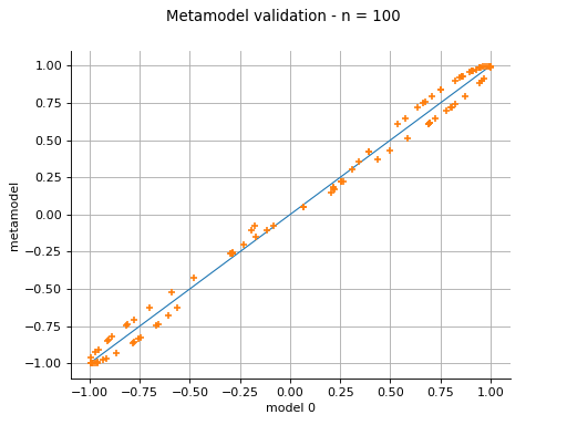
(Source code, png)

class MetaModelValidation(*args)¶

Scores a metamodel in order to perform its validation.

Parameters:

outputSample2-d sequence of float: The output validation sample, not used during the learning step.
metamodelPredictions: 2-d sequence of float: The output prediction sample from the metamodel.

Methods

`computeMeanSquaredError`()	Accessor to the mean squared error.
`computeR2Score`()	Compute the R2 score.
`drawValidation`()	Plot a model vs metamodel graph for visual validation.
`getClassName`()	Accessor to the object's name.
`getMetamodelPredictions`()	Accessor to the output predictions from the metamodel.
`getName`()	Accessor to the object's name.
`getOutputSample`()	Accessor to the output sample.
`getResidualDistribution`([smooth])	Compute the non parametric distribution of the residual sample.
`getResidualSample`()	Compute the residual sample.
`hasName`()	Test if the object is named.
`setName`(name)	Accessor to the object's name.

Notes

A MetaModelValidation object is used for the validation of a metamodel. For that purpose, a dataset independent of the learning step, is used to score the surrogate model. Its main functionalities are :

compute the coefficient of determination $R^2$ ;
get the residual sample and its non parametric distribution ;
draw a validation graph presenting the metamodel predictions against the model observations.

More details on this topic are presented in Validation and cross validation of metamodels.

Examples

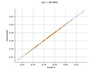
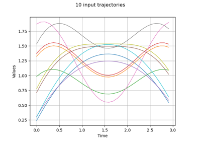
In this example, we introduce the sinus model and approximate it with a least squares metamodel. Then we validate this metamodel using a test sample.

>>> import openturns as ot
>>> from math import pi
>>> dist = ot.Uniform(-pi / 2, pi / 2)
>>> # Define the model
>>> model = ot.SymbolicFunction(['x'], ['sin(x)'])
>>> # We can build several types of models (kriging, polynomial chaos expansion, ...)
>>> # We use here a least squares expansion on canonical basis and compare
>>> # the metamodel with the model
>>> # Build the metamodel using a train sample
>>> x_train = dist.getSample(25)
>>> y_train = model(x_train)
>>> total_degree = 3
>>> polynomialCollection = [f'x^{degree + 1}' for degree in range(total_degree)]
>>> basis = ot.SymbolicFunction(['x'], polynomialCollection)
>>> designMatrix = basis(x_train)
>>> myLeastSquares = ot.LinearLeastSquares(designMatrix, y_train)
>>> myLeastSquares.run()
>>> leastSquaresModel = myLeastSquares.getMetaModel()
>>> metaModel = ot.ComposedFunction(leastSquaresModel, basis)
>>> # Validate the metamodel using a test sample
>>> x_test = dist.getSample(100)
>>> y_test = model(x_test)
>>> metamodelPredictions = metaModel(x_test)
>>> val = ot.MetaModelValidation(y_test, metamodelPredictions)
>>> # Compute the R2 score
>>> r2Score = val.computeR2Score()
>>> # Get the residual
>>> residual = val.getResidualSample()
>>> # Get the histogram of residuals
>>> histoResidual = val.getResidualDistribution(False)
>>> # Draw the validation graph
>>> graph = val.drawValidation()

__init__(*args)¶

computeMeanSquaredError()¶

Accessor to the mean squared error.

Returns:

meanSquaredErrorPoint: The mean squared error of each marginal output dimension.

Notes

The sample mean squared error is:

$\widehat{\operatorname{MSE}} = \frac{1}{n} \sum_{j=1}^{n} \left(y^{(j)} - \tilde{g}\left(\bdx^{(j)}\right)\right)^2$

where $n \in \Nset$ is the sample size, $\tilde{g}$ is the metamodel, $\{\bdx^{(j)} \in \Rset^{n_X}\}_{j = 1, ..., n}$ is the input experimental design and $\{y^{(j)} \in \Rset\}_{j = 1, ..., n}$ is the output of the model.

If the output is multi-dimensional, the same calculations are repeated separately for each output marginal $k$ for $k = 1, ..., n_y$ where $n_y \in \Nset$ is the output dimension.

computeR2Score()¶

Compute the R2 score.

Returns:

r2ScorePoint: The coefficient of determination R2

Notes

The coefficient of determination $R^2$ is the fraction of the variance of the output explained by the metamodel. It is defined as:

$R^2 = 1 - \operatorname{FVU}$

where $\operatorname{FVU}$ is the fraction of unexplained variance:

$\operatorname{FVU} = \frac{\operatorname{MSE}(\tilde{g}) }{\Var{Y}}$

where $Y = g(\bdX)$ is the output of the physical model $g$ , $\Var{Y}$ is the variance of the output and $\operatorname{MSE}$ is the mean squared error of the metamodel:

$\operatorname{MSE}(\tilde{g}) = \Expect{\left(g(\bdX) - \tilde{g}(\bdX) \right)^2}.$

The sample $R^2$ is:

$\hat{R}^2 = 1 - \frac{\frac{1}{n} \sum_{j=1}^{n} \left(y^{(j)} - \tilde{g}\left(\bdx^{(j)}\right)\right)^2}{\hat{\sigma}^2_Y}$

where $n \in \Nset$ is the sample size, $\tilde{g}$ is the metamodel, $\left\{\bdx^{(j)} \in \Rset^{n_X}\right\}_{j = 1, ..., n}$ is the input experimental design, $\left\{y^{(j)} \in \Rset\right\}_{j = 1, ..., n}$ is the output of the model and $\hat{\sigma}^2_Y$ is the sample variance of the output:

$\hat{\sigma}^2_Y = \frac{1}{n - 1} \sum_{j=1}^{n} \left(y^{(j)} - \overline{y}\right)^2$

where $\overline{y}$ is the output sample mean:

$\overline{y} = \frac{1}{n} \sum_{j=1}^{n} y^{(j)}.$

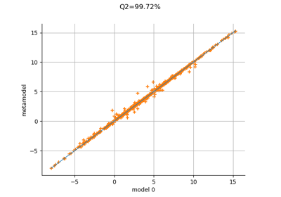
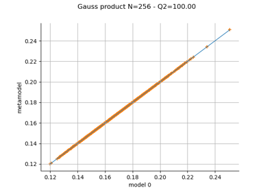
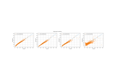
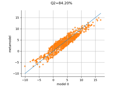
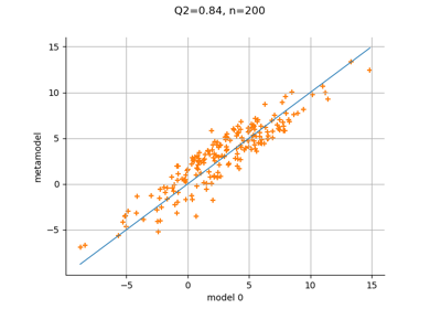
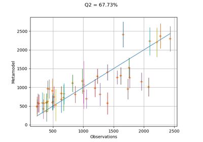
drawValidation()¶

Plot a model vs metamodel graph for visual validation.

Returns:

graphGridLayout: The visual validation graph.

Notes

The plot presents the metamodel predictions depending on the model observations. If the points are close to the diagonal line of the plot, then the metamodel validation is satisfactory. Points which are far away from the diagonal represent outputs for which the metamodel is not accurate.

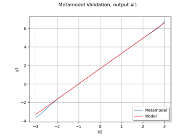
If the output is multi-dimensional, the graph has 1 row and $n_y \in \Nset$ columns, where $n_y$ is the output dimension.

getClassName()¶

Accessor to the object’s name.

Returns:

class_namestr: The object class name (object.__class__.__name__).

getMetamodelPredictions()¶

Accessor to the output predictions from the metamodel.

Returns:

outputMetamodelSampleSample: Output sample of the metamodel.

getName()¶

Accessor to the object’s name.

Returns:

namestr: The name of the object.

getOutputSample()¶

Accessor to the output sample.

Returns:

outputSampleSample: Output sample of a model evaluated apart.

getResidualDistribution(smooth=True)¶

Compute the non parametric distribution of the residual sample.

Parameters:

smoothbool: Tells if distribution is smooth (true) or not. Default argument is true.

Returns:

residualDistributionDistribution: The residual distribution.

Notes

The residual distribution is built thanks to KernelSmoothing if smooth argument is true. Otherwise, an histogram distribution is returned, thanks to HistogramFactory.

getResidualSample()¶

Compute the residual sample.

Returns:

residualSample: The residual sample.

Notes

The residual sample is given by :

$r^{(j)} = y^{(j)} - \tilde{g}\left(\vect{x}^{(j)}\right)$

for $j = 1, ..., n$ where $n \in \Nset$ is the sample size, $y^{(j)}$ is the model observation, $\tilde{g}$ is the metamodel and $\vect{x}^{(j)}$ is the $j$ -th input observation.

If the output is multi-dimensional, the residual sample has dimension $n_y \in \Nset$ , where $n_y$ is the output dimension.

hasName()¶

Test if the object is named.

Returns: