FMUPointToFieldFunction basics

otfmi.FMUPointToFieldFunction wraps the FMU into an openturns.PointToFieldFunction object. This kind of function accepts openturns.Point or openturns.Sample as inputs, and outputs a openturns.Sample or a set of openturns.Field.

---

First, retrieve the path to epid.fmu. Recall the deviation model is dynamic, i.e. its output evolves over time.

import openturns as ot
import otfmi.example.utility
import matplotlib.pyplot as plt
import openturns.viewer as viewer


path_fmu = otfmi.example.utility.get_path_fmu("epid")

Define the time grid for the FMU’s output. The last value of the time grid, here 10., will define the FMU stop time for simulation.

mesh = ot.RegularGrid(0.0, 0.1, 2000)
meshSample = mesh.getVertices()
print(meshSample)

       [ t     ]
   0 : [   0   ]
   1 : [   0.1 ]
   2 : [   0.2 ]
...
1997 : [ 199.7 ]
1998 : [ 199.8 ]
1999 : [ 199.9 ]

Note

The FMU solver uses its own time grid for simulation. The FMU output is then interpolated on the user-provided time grid.

Wrap the FMU in an openturns.PointToFieldFunction object:

function = otfmi.FMUPointToFieldFunction(
    mesh,
    path_fmu,
    inputs_fmu=["infection_rate"],
    outputs_fmu=["infected"],
    start_time=0.0,
    final_time=200.0,
)
print(type(function))

<class 'openturns.func.PointToFieldFunction'>

Note

The start and final times must define an interval comprising the mesh. Setting manually the start and final times is recommended to avoid uncontrolled simulation duration.

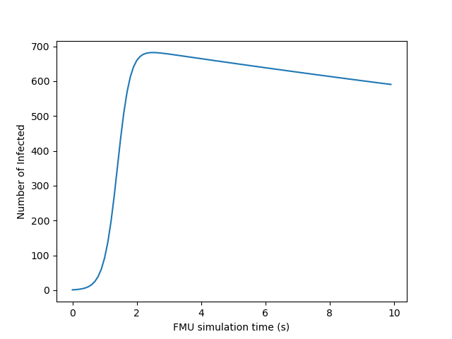
Simulate the function on an input openturns.Point yields an output openturns.Sample, corresponding to the output evolution over time:

inputPoint = ot.Point([2.0])
outputSample = function(inputPoint)

plt.xlabel("FMU simulation time (s)")
plt.ylabel("Number of Infected")
plt.plot(meshSample, outputSample)
plt.show()

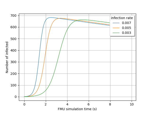
Simulate the function on a input openturns.Sample yields a set of fields called openturns.ProcessSample:

inputSample = ot.Sample([[2.0], [2.25], [2.5]])
outputProcessSample = function(inputSample)
print(outputProcessSample)

[field 0:
       [ t             infected      ]
   0 : [   0             1           ]
   1 : [   0.1           1.14974     ]
   2 : [   0.2           1.29948     ]
...
1997 : [ 199.7           1.46173e-42 ]
1998 : [ 199.8           1.38833e-42 ]
1999 : [ 199.9           1.31492e-42 ]
field 1:
       [ t             infected      ]
   0 : [   0             1           ]
   1 : [   0.1           1.17471     ]
   2 : [   0.2           1.34941     ]
...
1997 : [ 199.7           7.73327e-44 ]
1998 : [ 199.8           7.33573e-44 ]
1999 : [ 199.9           6.9382e-44  ]
field 2:
       [ t             infected      ]
   0 : [   0             1           ]
   1 : [   0.1           1.19967     ]
   2 : [   0.2           1.39934     ]
...
1997 : [ 199.7           1.38086e-44 ]
1998 : [ 199.8           1.30896e-44 ]
1999 : [ 199.9           1.23707e-44 ]]

Visualize the time evolution of the infected over time, depending on the ìnfection_rate` value:

gridLayout = outputProcessSample.draw()
graph = gridLayout.getGraph(0, 0)
graph.setTitle("")
graph.setXTitle("FMU simulation time (s)")
graph.setYTitle("Number of infected")
graph.setLegends([str(line[0]) for line in inputSample])
view = viewer.View(graph, legend_kw={"title": "infection rate"})
view.ShowAll()