KrigingResult
- class KrigingResult(*args)
Kriging result.
- Available constructors:
KrigingResult(inputSample, outputSample, metaModel, residuals, relativeErrors, basis, trendCoefficients, covarianceModel, covarianceCoefficients)
KrigingResult(inputSample, outputSample, metaModel, residuals, relativeErrors, basis, trendCoefficients, covarianceModel, covarianceCoefficients, covarianceCholeskyFactor, covarianceHMatrix)
- Parameters:
- inputSample, outputSample2-d sequence of float
The samples
 and
and  .
.- metaModel
Function The meta model:
 , defined in (3).
- residuals
Point The residual errors.
- relativeErrors
Point The relative errors.
- basis
Basis Functional basis of size
 :
:  for each
 ![l \in [1, b]](data:image/svg+xml;base64,PD94bWwgdmVyc2lvbj0nMS4wJyBlbmNvZGluZz0nVVRGLTgnPz4KPCEtLSBUaGlzIGZpbGUgd2FzIGdlbmVyYXRlZCBieSBkdmlzdmdtIDMuNC4yIC0tPgo8c3ZnIHZlcnNpb249JzEuMScgeG1sbnM9J2h0dHA6Ly93d3cudzMub3JnLzIwMDAvc3ZnJyB4bWxuczp4bGluaz0naHR0cDovL3d3dy53My5vcmcvMTk5OS94bGluaycgd2lkdGg9JzQwLjkzOTE4M3B0JyBoZWlnaHQ9JzExLjk1NTE2OHB0JyB2aWV3Qm94PScwIC04Ljk2NjM3NiA0MC45MzkxODMgMTEuOTU1MTY4Jz4KPGRlZnM+CjxwYXRoIGlkPSdnMi00OScgZD0nTTMuNDQzMDg4LTcuNjYzMjYzQzMuNDQzMDg4LTcuOTM4MjMyIDMuNDQzMDg4LTcuOTUwMTg3IDMuMjAzOTg1LTcuOTUwMTg3QzIuOTE3MDYxLTcuNjI3Mzk3IDIuMzE5MzAzLTcuMTg1MDU2IDEuMDg3OTItNy4xODUwNTZWLTYuODM4MzU2QzEuMzYyODg5LTYuODM4MzU2IDEuOTYwNjQ4LTYuODM4MzU2IDIuNjE4MTgyLTcuMTQ5MTkxVi0uOTIwNTQ4QzIuNjE4MTgyLS40OTAxNjIgMi41ODIzMTYtLjM0NjcgMS41MzAyNjItLjM0NjdIMS4xNTk2NTFWMEMxLjQ4MjQ0MS0uMDIzOTEgMi42NDIwOTItLjAyMzkxIDMuMDM2NjEzLS4wMjM5MVM0LjU3ODgyOS0uMDIzOTEgNC45MDE2MTkgMFYtLjM0NjdINC41MzEwMDlDMy40Nzg5NTQtLjM0NjcgMy40NDMwODgtLjQ5MDE2MiAzLjQ0MzA4OC0uOTIwNTQ4Vi03LjY2MzI2M1onLz4KPHBhdGggaWQ9J2cyLTkxJyBkPSdNMi45ODg3OTIgMi45ODg3OTJWMi41NDY0NTFIMS44MjkxNDFWLTguNTI0MDM1SDIuOTg4NzkyVi04Ljk2NjM3NkgxLjM4NjhWMi45ODg3OTJIMi45ODg3OTJaJy8+CjxwYXRoIGlkPSdnMi05MycgZD0nTTEuODUzMDUxLTguOTY2Mzc2SC4yNTEwNTlWLTguNTI0MDM1SDEuNDEwNzFWMi41NDY0NTFILjI1MTA1OVYyLjk4ODc5MkgxLjg1MzA1MVYtOC45NjYzNzZaJy8+CjxwYXRoIGlkPSdnMC01MCcgZD0nTTYuNTUxNDMyLTIuNzQ5Njg5QzYuNzU0NjctMi43NDk2ODkgNi45Njk4NjMtMi43NDk2ODkgNi45Njk4NjMtMi45ODg3OTJTNi43NTQ2Ny0zLjIyNzg5NSA2LjU1MTQzMi0zLjIyNzg5NUgxLjQ4MjQ0MUMxLjYyNTkwMy00LjgyOTg4OCAzLjAwMDc0Ny01Ljk3NzU4NCA0LjY4NjQyNi01Ljk3NzU4NEg2LjU1MTQzMkM2Ljc1NDY3LTUuOTc3NTg0IDYuOTY5ODYzLTUuOTc3NTg0IDYuOTY5ODYzLTYuMjE2Njg3UzYuNzU0NjctNi40NTU3OTEgNi41NTE0MzItNi40NTU3OTFINC42NjI1MTZDMi42MTgxODItNi40NTU3OTEgLjk5MjI3OS00LjkwMTYxOSAuOTkyMjc5LTIuOTg4NzkyUzIuNjE4MTgyIC40NzgyMDcgNC42NjI1MTYgLjQ3ODIwN0g2LjU1MTQzMkM2Ljc1NDY3IC40NzgyMDcgNi45Njk4NjMgLjQ3ODIwNyA2Ljk2OTg2MyAuMjM5MTAzUzYuNzU0NjcgMCA2LjU1MTQzMiAwSDQuNjg2NDI2QzMuMDAwNzQ3IDAgMS42MjU5MDMtMS4xNDc2OTYgMS40ODI0NDEtMi43NDk2ODlINi41NTE0MzJaJy8+CjxwYXRoIGlkPSdnMS01OScgZD0nTTIuMzMxMjU4IC4wNDc4MjFDMi4zMzEyNTgtLjY0NTU3OSAyLjEwNDExLTEuMTU5NjUxIDEuNjEzOTQ4LTEuMTU5NjUxQzEuMjMxMzgyLTEuMTU5NjUxIDEuMDQwMS0uODQ4ODE3IDEuMDQwMS0uNTg1ODAzUzEuMjE5NDI3IDAgMS42MjU5MDMgMEMxLjc4MTMyIDAgMS45MTI4MjctLjA0NzgyMSAyLjAyMDQyMy0uMTU1NDE3QzIuMDQ0MzM0LS4xNzkzMjggMi4wNTYyODktLjE3OTMyOCAyLjA2ODI0NC0uMTc5MzI4QzIuMDkyMTU0LS4xNzkzMjggMi4wOTIxNTQtLjAxMTk1NSAyLjA5MjE1NCAuMDQ3ODIxQzIuMDkyMTU0IC40NDIzNDEgMi4wMjA0MjMgMS4yMTk0MjcgMS4zMjcwMjQgMS45OTY1MTNDMS4xOTU1MTcgMi4xMzk5NzUgMS4xOTU1MTcgMi4xNjM4ODUgMS4xOTU1MTcgMi4xODc3OTZDMS4xOTU1MTcgMi4yNDc1NzIgMS4yNTUyOTMgMi4zMDczNDcgMS4zMTUwNjggMi4zMDczNDdDMS40MTA3MSAyLjMwNzM0NyAyLjMzMTI1OCAxLjQyMjY2NSAyLjMzMTI1OCAuMDQ3ODIxWicvPgo8cGF0aCBpZD0nZzEtOTgnIGQ9J00yLjc2MTY0NC03Ljk5ODAwN0MyLjc3MzU5OS04LjA0NTgyOCAyLjc5NzUwOS04LjExNzU1OSAyLjc5NzUwOS04LjE3NzMzNUMyLjc5NzUwOS04LjI5Njg4NyAyLjY3Nzk1OC04LjI5Njg4NyAyLjY1NDA0Ny04LjI5Njg4N0MyLjY0MjA5Mi04LjI5Njg4NyAyLjIxMTcwNi04LjI2MTAyMSAxLjk5NjUxMy04LjIzNzExMUMxLjc5MzI3NS04LjIyNTE1NiAxLjYxMzk0OC04LjIwMTI0NSAxLjM5ODc1NS04LjE4OTI5QzEuMTExODMxLTguMTY1MzggMS4wMjgxNDQtOC4xNTM0MjUgMS4wMjgxNDQtNy45MzgyMzJDMS4wMjgxNDQtNy44MTg2OCAxLjE0NzY5Ni03LjgxODY4IDEuMjY3MjQ4LTcuODE4NjhDMS44NzY5NjEtNy44MTg2OCAxLjg3Njk2MS03LjcxMTA4MyAxLjg3Njk2MS03LjU5MTUzMkMxLjg3Njk2MS03LjUwNzg0NiAxLjc4MTMyLTcuMTYxMTQ2IDEuNzMzNDk5LTYuOTQ1OTUzTDEuNDQ2NTc1LTUuNzk4MjU3QzEuMzI3MDI0LTUuMzIwMDUgLjY0NTU3OS0yLjYwNjIyNyAuNTk3NzU4LTIuMzkxMDM0Qy41Mzc5ODMtMi4wOTIxNTQgLjUzNzk4My0xLjg4ODkxNyAuNTM3OTgzLTEuNzMzNDk5Qy41Mzc5ODMtLjUxNDA3MiAxLjIxOTQyNyAuMTE5NTUyIDEuOTk2NTEzIC4xMTk1NTJDMy4zODMzMTMgLjExOTU1MiA0LjgxNzkzMy0xLjY2MTc2OCA0LjgxNzkzMy0zLjM5NTI2OEM0LjgxNzkzMy00LjQ5NTE0MyA0LjE5NjI2NC01LjI3MjIyOSAzLjI5OTYyNi01LjI3MjIyOUMyLjY3Nzk1OC01LjI3MjIyOSAyLjExNjA2NS00Ljc1ODE1NyAxLjg4ODkxNy00LjUxOTA1NEwyLjc2MTY0NC03Ljk5ODAwN1pNMi4wMDg0NjgtLjExOTU1MkMxLjYyNTkwMy0uMTE5NTUyIDEuMjA3NDcyLS40MDY0NzYgMS4yMDc0NzItMS4zMzg5NzlDMS4yMDc0NzItMS43MzM0OTkgMS4yNDMzMzctMS45NjA2NDggMS40NTg1MzEtMi43OTc1MDlDMS40OTQzOTYtMi45NTI5MjcgMS42ODU2NzktMy43MTgwNTcgMS43MzM0OTktMy44NzM0NzRDMS43NTc0MS0zLjk2OTExNiAyLjQ2Mjc2NS01LjAzMzEyNiAzLjI3NTcxNi01LjAzMzEyNkMzLjgwMTc0My01LjAzMzEyNiA0LjA0MDg0Ny00LjUwNzA5OCA0LjA0MDg0Ny0zLjg4NTQzQzQuMDQwODQ3LTMuMzExNTgyIDMuNzA2MTAyLTEuOTYwNjQ4IDMuNDA3MjIzLTEuMzM4OTc5QzMuMTA4MzQ0LS42OTM0IDIuNTU4NDA2LS4xMTk1NTIgMi4wMDg0NjgtLjExOTU1MlonLz4KPHBhdGggaWQ9J2cxLTEwOCcgZD0nTTMuMDM2NjEzLTcuOTk4MDA3QzMuMDQ4NTY4LTguMDQ1ODI4IDMuMDcyNDc4LTguMTE3NTU5IDMuMDcyNDc4LTguMTc3MzM1QzMuMDcyNDc4LTguMjk2ODg3IDIuOTUyOTI3LTguMjk2ODg3IDIuOTI5MDE2LTguMjk2ODg3QzIuOTE3MDYxLTguMjk2ODg3IDIuNDg2Njc1LTguMjYxMDIxIDIuMjcxNDgyLTguMjM3MTExQzIuMDY4MjQ0LTguMjI1MTU2IDEuODg4OTE3LTguMjAxMjQ1IDEuNjczNzI0LTguMTg5MjlDMS4zODY4LTguMTY1MzggMS4zMDMxMTMtOC4xNTM0MjUgMS4zMDMxMTMtNy45MzgyMzJDMS4zMDMxMTMtNy44MTg2OCAxLjQyMjY2NS03LjgxODY4IDEuNTQyMjE3LTcuODE4NjhDMi4xNTE5My03LjgxODY4IDIuMTUxOTMtNy43MTEwODMgMi4xNTE5My03LjU5MTUzMkMyLjE1MTkzLTcuNTQzNzExIDIuMTUxOTMtNy41MTk4MDEgMi4wOTIxNTQtNy4zMDQ2MDhMLjYwOTcxNC0xLjM3NDg0NEMuNTczODQ4LTEuMjQzMzM3IC41NDk5MzgtMS4xNDc2OTYgLjU0OTkzOC0uOTU2NDEzQy41NDk5MzgtLjM1ODY1NSAuOTkyMjc5IC4xMTk1NTIgMS42MDE5OTMgLjExOTU1MkMxLjk5NjUxMyAuMTE5NTUyIDIuMjU5NTI3LS4xNDM0NjIgMi40NTA4MDktLjUxNDA3MkMyLjY1NDA0Ny0uOTA4NTkzIDIuODIxNDItMS42NjE3NjggMi44MjE0Mi0xLjcwOTU4OUMyLjgyMTQyLTEuNzY5MzY1IDIuNzczNTk5LTEuODE3MTg2IDIuNzAxODY4LTEuODE3MTg2QzIuNTk0MjcxLTEuODE3MTg2IDIuNTgyMzE2LTEuNzU3NDEgMi41MzQ0OTYtMS41NzgwODJDMi4zMTkzMDMtLjc1MzE3NiAyLjEwNDExLS4xMTk1NTIgMS42MjU5MDMtLjExOTU1MkMxLjI2NzI0OC0uMTE5NTUyIDEuMjY3MjQ4LS41MDIxMTcgMS4yNjcyNDgtLjY2OTQ4OUMxLjI2NzI0OC0uNzE3MzEgMS4yNjcyNDgtLjk2ODM2OSAxLjM1MDkzNC0xLjMwMzExM0wzLjAzNjYxMy03Ljk5ODAwN1onLz4KPC9kZWZzPgo8ZyBpZD0ncGFnZTEnPgo8dXNlIHg9JzAnIHk9JzAnIHhsaW5rOmhyZWY9JyNnMS0xMDgnLz4KPHVzZSB4PSc3LjA3MDYzOCcgeT0nMCcgeGxpbms6aHJlZj0nI2cwLTUwJy8+Cjx1c2UgeD0nMTguMzYxNjA2JyB5PScwJyB4bGluazpocmVmPScjZzItOTEnLz4KPHVzZSB4PScyMS42MTMyNjcnIHk9JzAnIHhsaW5rOmhyZWY9JyNnMi00OScvPgo8dXNlIHg9JzI3LjQ2NjI1NycgeT0nMCcgeGxpbms6aHJlZj0nI2cxLTU5Jy8+Cjx1c2UgeD0nMzIuNzEwNDE2JyB5PScwJyB4bGluazpocmVmPScjZzEtOTgnLz4KPHVzZSB4PSczNy42ODc1MjInIHk9JzAnIHhsaW5rOmhyZWY9JyNnMi05MycvPgo8L2c+Cjwvc3ZnPgo8IS0tIERFUFRIPTQgLS0+) .
Its size should be equal to zero if the trend is not estimated.
.
Its size should be equal to zero if the trend is not estimated.- trendCoefficients
Point The trend coefficients vectors
 stored as a Point.
- covarianceModel
CovarianceModel Covariance function of the Gaussian process.
- covarianceCoefficients2-d sequence of float
The
 defined in (2).
- covarianceCholeskyFactor
TriangularMatrix The Cholesky factor
 of
of  .
.- covarianceHMatrix
HMatrix The hmat implementation of
.
Methods
getBasis()Accessor to the functional basis.
Accessor to the object's name.
getConditionalCovariance(*args)Compute the conditional covariance of the Gaussian process on a point (or several points).
Compute the conditional covariance of the Gaussian process on a point (or several points).
Compute the conditional variance of the Gaussian process on a point (or several points).
getConditionalMean(*args)Compute the conditional mean of the Gaussian process on a point or a sample of points.
Accessor to the covariance coefficients.
Accessor to the covariance model.
Accessor to the input sample.
Accessor to the metamodel.
getName()Accessor to the object's name.
Accessor to the output sample.
Accessor to the relative errors.
Accessor to the residuals.
Accessor to the trend coefficients.
hasName()Test if the object is named.
setInputSample(sampleX)Accessor to the input sample.
setMetaModel(metaModel)Accessor to the metamodel.
setName(name)Accessor to the object's name.
setOutputSample(sampleY)Accessor to the output sample.
setRelativeErrors(relativeErrors)Accessor to the relative errors.
setResiduals(residuals)Accessor to the residuals.
Notes
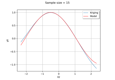
The Kriging meta model
 is defined by:
(1)

where
 is the condition
  for each
 ![k \in [1, N]](data:image/svg+xml;base64,PD94bWwgdmVyc2lvbj0nMS4wJyBlbmNvZGluZz0nVVRGLTgnPz4KPCEtLSBUaGlzIGZpbGUgd2FzIGdlbmVyYXRlZCBieSBkdmlzdmdtIDMuNC4yIC0tPgo8c3ZnIHZlcnNpb249JzEuMScgeG1sbnM9J2h0dHA6Ly93d3cudzMub3JnLzIwMDAvc3ZnJyB4bWxuczp4bGluaz0naHR0cDovL3d3dy53My5vcmcvMTk5OS94bGluaycgd2lkdGg9JzQ5LjMyNDM4M3B0JyBoZWlnaHQ9JzExLjk1NTE2OHB0JyB2aWV3Qm94PScwIC04Ljk2NjM3NiA0OS4zMjQzODMgMTEuOTU1MTY4Jz4KPGRlZnM+CjxwYXRoIGlkPSdnMi00OScgZD0nTTMuNDQzMDg4LTcuNjYzMjYzQzMuNDQzMDg4LTcuOTM4MjMyIDMuNDQzMDg4LTcuOTUwMTg3IDMuMjAzOTg1LTcuOTUwMTg3QzIuOTE3MDYxLTcuNjI3Mzk3IDIuMzE5MzAzLTcuMTg1MDU2IDEuMDg3OTItNy4xODUwNTZWLTYuODM4MzU2QzEuMzYyODg5LTYuODM4MzU2IDEuOTYwNjQ4LTYuODM4MzU2IDIuNjE4MTgyLTcuMTQ5MTkxVi0uOTIwNTQ4QzIuNjE4MTgyLS40OTAxNjIgMi41ODIzMTYtLjM0NjcgMS41MzAyNjItLjM0NjdIMS4xNTk2NTFWMEMxLjQ4MjQ0MS0uMDIzOTEgMi42NDIwOTItLjAyMzkxIDMuMDM2NjEzLS4wMjM5MVM0LjU3ODgyOS0uMDIzOTEgNC45MDE2MTkgMFYtLjM0NjdINC41MzEwMDlDMy40Nzg5NTQtLjM0NjcgMy40NDMwODgtLjQ5MDE2MiAzLjQ0MzA4OC0uOTIwNTQ4Vi03LjY2MzI2M1onLz4KPHBhdGggaWQ9J2cyLTkxJyBkPSdNMi45ODg3OTIgMi45ODg3OTJWMi41NDY0NTFIMS44MjkxNDFWLTguNTI0MDM1SDIuOTg4NzkyVi04Ljk2NjM3NkgxLjM4NjhWMi45ODg3OTJIMi45ODg3OTJaJy8+CjxwYXRoIGlkPSdnMi05MycgZD0nTTEuODUzMDUxLTguOTY2Mzc2SC4yNTEwNTlWLTguNTI0MDM1SDEuNDEwNzFWMi41NDY0NTFILjI1MTA1OVYyLjk4ODc5MkgxLjg1MzA1MVYtOC45NjYzNzZaJy8+CjxwYXRoIGlkPSdnMC01MCcgZD0nTTYuNTUxNDMyLTIuNzQ5Njg5QzYuNzU0NjctMi43NDk2ODkgNi45Njk4NjMtMi43NDk2ODkgNi45Njk4NjMtMi45ODg3OTJTNi43NTQ2Ny0zLjIyNzg5NSA2LjU1MTQzMi0zLjIyNzg5NUgxLjQ4MjQ0MUMxLjYyNTkwMy00LjgyOTg4OCAzLjAwMDc0Ny01Ljk3NzU4NCA0LjY4NjQyNi01Ljk3NzU4NEg2LjU1MTQzMkM2Ljc1NDY3LTUuOTc3NTg0IDYuOTY5ODYzLTUuOTc3NTg0IDYuOTY5ODYzLTYuMjE2Njg3UzYuNzU0NjctNi40NTU3OTEgNi41NTE0MzItNi40NTU3OTFINC42NjI1MTZDMi42MTgxODItNi40NTU3OTEgLjk5MjI3OS00LjkwMTYxOSAuOTkyMjc5LTIuOTg4NzkyUzIuNjE4MTgyIC40NzgyMDcgNC42NjI1MTYgLjQ3ODIwN0g2LjU1MTQzMkM2Ljc1NDY3IC40NzgyMDcgNi45Njk4NjMgLjQ3ODIwNyA2Ljk2OTg2MyAuMjM5MTAzUzYuNzU0NjcgMCA2LjU1MTQzMiAwSDQuNjg2NDI2QzMuMDAwNzQ3IDAgMS42MjU5MDMtMS4xNDc2OTYgMS40ODI0NDEtMi43NDk2ODlINi41NTE0MzJaJy8+CjxwYXRoIGlkPSdnMS01OScgZD0nTTIuMzMxMjU4IC4wNDc4MjFDMi4zMzEyNTgtLjY0NTU3OSAyLjEwNDExLTEuMTU5NjUxIDEuNjEzOTQ4LTEuMTU5NjUxQzEuMjMxMzgyLTEuMTU5NjUxIDEuMDQwMS0uODQ4ODE3IDEuMDQwMS0uNTg1ODAzUzEuMjE5NDI3IDAgMS42MjU5MDMgMEMxLjc4MTMyIDAgMS45MTI4MjctLjA0NzgyMSAyLjAyMDQyMy0uMTU1NDE3QzIuMDQ0MzM0LS4xNzkzMjggMi4wNTYyODktLjE3OTMyOCAyLjA2ODI0NC0uMTc5MzI4QzIuMDkyMTU0LS4xNzkzMjggMi4wOTIxNTQtLjAxMTk1NSAyLjA5MjE1NCAuMDQ3ODIxQzIuMDkyMTU0IC40NDIzNDEgMi4wMjA0MjMgMS4yMTk0MjcgMS4zMjcwMjQgMS45OTY1MTNDMS4xOTU1MTcgMi4xMzk5NzUgMS4xOTU1MTcgMi4xNjM4ODUgMS4xOTU1MTcgMi4xODc3OTZDMS4xOTU1MTcgMi4yNDc1NzIgMS4yNTUyOTMgMi4zMDczNDcgMS4zMTUwNjggMi4zMDczNDdDMS40MTA3MSAyLjMwNzM0NyAyLjMzMTI1OCAxLjQyMjY2NSAyLjMzMTI1OCAuMDQ3ODIxWicvPgo8cGF0aCBpZD0nZzEtNzgnIGQ9J004Ljg0NjgyNC02LjkxMDA4N0M4Ljk3ODMzMS03LjQyNDE1OSA5LjE2OTYxNC03Ljc4MjgxNCAxMC4wNzgyMDctNy44MTg2OEMxMC4xMTQwNzItNy44MTg2OCAxMC4yNTc1MzQtNy44MzA2MzUgMTAuMjU3NTM0LTguMDMzODczQzEwLjI1NzUzNC04LjE2NTM4IDEwLjE0OTkzOC04LjE2NTM4IDEwLjEwMjExNy04LjE2NTM4QzkuODYzMDE0LTguMTY1MzggOS4yNTMzLTguMTQxNDY5IDkuMDE0MTk3LTguMTQxNDY5SDguNDQwMzQ5QzguMjcyOTc2LTguMTQxNDY5IDguMDU3NzgzLTguMTY1MzggNy44OTA0MTEtOC4xNjUzOEM3LjgxODY4LTguMTY1MzggNy42NzUyMTgtOC4xNjUzOCA3LjY3NTIxOC03LjkzODIzMkM3LjY3NTIxOC03LjgxODY4IDcuNzcwODU5LTcuODE4NjggNy44NTQ1NDUtNy44MTg2OEM4LjU3MTg1Ni03Ljc5NDc3IDguNjE5Njc2LTcuNTE5ODAxIDguNjE5Njc2LTcuMzA0NjA4QzguNjE5Njc2LTcuMTk3MDExIDguNjA3NzIxLTcuMTYxMTQ2IDguNTcxODU2LTYuOTkzNzczTDcuMjIwOTIyLTEuNjAxOTkzTDQuNjYyNTE2LTcuOTYyMTQyQzQuNTc4ODI5LTguMTUzNDI1IDQuNTY2ODc0LTguMTY1MzggNC4zMDM4NjEtOC4xNjUzOEgyLjg0NTMzQzIuNjA2MjI3LTguMTY1MzggMi40OTg2My04LjE2NTM4IDIuNDk4NjMtNy45MzgyMzJDMi40OTg2My03LjgxODY4IDIuNTgyMzE2LTcuODE4NjggMi44MDk0NjUtNy44MTg2OEMyLjg2OTI0LTcuODE4NjggMy41NzQ1OTUtNy44MTg2OCAzLjU3NDU5NS03LjcxMTA4M0MzLjU3NDU5NS03LjY4NzE3MyAzLjU1MDY4NS03LjU5MTUzMiAzLjUzODczLTcuNTU1NjY2TDEuOTQ4NjkyLTEuMjE5NDI3QzEuODA1MjMtLjYzMzYyNCAxLjUxODMwNi0uMzgyNTY1IC43MjkyNjUtLjM0NjdDLjY2OTQ4OS0uMzQ2NyAuNTQ5OTM4LS4zMzQ3NDUgLjU0OTkzOC0uMTE5NTUyQy41NDk5MzggMCAuNjY5NDg5IDAgLjcwNTM1NSAwQy45NDQ0NTggMCAxLjU1NDE3Mi0uMDIzOTEgMS43OTMyNzUtLjAyMzkxSDIuMzY3MTIzQzIuNTM0NDk2LS4wMjM5MSAyLjczNzczMyAwIDIuOTA1MTA2IDBDMi45ODg3OTIgMCAzLjEyMDI5OSAwIDMuMTIwMjk5LS4yMjcxNDhDMy4xMjAyOTktLjMzNDc0NSAzLjAwMDc0Ny0uMzQ2NyAyLjk1MjkyNy0uMzQ2N0MyLjU1ODQwNi0uMzU4NjU1IDIuMTc1ODQxLS40MzAzODYgMi4xNzU4NDEtLjg2MDc3MkMyLjE3NTg0MS0uOTU2NDEzIDIuMTk5NzUxLTEuMDY0MDEgMi4yMjM2NjEtMS4xNTk2NTFMMy44Mzc2MDktNy41NTU2NjZDMy45MDkzNC03LjQzNjExNSAzLjkwOTM0LTcuNDEyMjA0IDMuOTU3MTYxLTcuMzA0NjA4TDYuODAyNDkxLS4yMTUxOTNDNi44NjIyNjctLjA3MTczMSA2Ljg4NjE3NyAwIDYuOTkzNzczIDBDNy4xMTMzMjUgMCA3LjEyNTI4LS4wMzU4NjYgNy4xNzMxMDEtLjIzOTEwM0w4Ljg0NjgyNC02LjkxMDA4N1onLz4KPHBhdGggaWQ9J2cxLTEwNycgZD0nTTMuMzU5NDAyLTcuOTk4MDA3QzMuMzcxMzU3LTguMDQ1ODI4IDMuMzk1MjY4LTguMTE3NTU5IDMuMzk1MjY4LTguMTc3MzM1QzMuMzk1MjY4LTguMjk2ODg3IDMuMjc1NzE2LTguMjk2ODg3IDMuMjUxODA2LTguMjk2ODg3QzMuMjM5ODUxLTguMjk2ODg3IDIuODA5NDY1LTguMjYxMDIxIDIuNTk0MjcxLTguMjM3MTExQzIuMzkxMDM0LTguMjI1MTU2IDIuMjExNzA2LTguMjAxMjQ1IDEuOTk2NTEzLTguMTg5MjlDMS43MDk1ODktOC4xNjUzOCAxLjYyNTkwMy04LjE1MzQyNSAxLjYyNTkwMy03LjkzODIzMkMxLjYyNTkwMy03LjgxODY4IDEuNzQ1NDU1LTcuODE4NjggMS44NjUwMDYtNy44MTg2OEMyLjQ3NDcyLTcuODE4NjggMi40NzQ3Mi03LjcxMTA4MyAyLjQ3NDcyLTcuNTkxNTMyQzIuNDc0NzItNy41NDM3MTEgMi40NzQ3Mi03LjUxOTgwMSAyLjQxNDk0NC03LjMwNDYwOEwuNzA1MzU1LS40NjYyNTJDLjY1NzUzNC0uMjg2OTI0IC42NTc1MzQtLjI2MzAxNCAuNjU3NTM0LS4xOTEyODNDLjY1NzUzNCAuMDcxNzMxIC44NjA3NzIgLjExOTU1MiAuOTgwMzI0IC4xMTk1NTJDMS4zMTUwNjggLjExOTU1MiAxLjM4NjgtLjE0MzQ2MiAxLjQ4MjQ0MS0uNTE0MDcyTDIuMDQ0MzM0LTIuNzQ5Njg5QzIuOTA1MTA2LTIuNjU0MDQ3IDMuNDE5MTc4LTIuMjk1MzkyIDMuNDE5MTc4LTEuNzIxNTQ0QzMuNDE5MTc4LTEuNjQ5ODEzIDMuNDE5MTc4LTEuNjAxOTkzIDMuMzgzMzEzLTEuNDIyNjY1QzMuMzM1NDkyLTEuMjQzMzM3IDMuMzM1NDkyLTEuMDk5ODc1IDMuMzM1NDkyLTEuMDQwMUMzLjMzNTQ5Mi0uMzQ2NyAzLjc4OTc4OCAuMTE5NTUyIDQuMzk5NTAyIC4xMTk1NTJDNC45NDk0NCAuMTE5NTUyIDUuMjM2MzY0LS4zODI1NjUgNS4zMzIwMDUtLjU0OTkzOEM1LjU4MzA2NC0uOTkyMjc5IDUuNzM4NDgxLTEuNjYxNzY4IDUuNzM4NDgxLTEuNzA5NTg5QzUuNzM4NDgxLTEuNzY5MzY1IDUuNjkwNjYtMS44MTcxODYgNS42MTg5MjktMS44MTcxODZDNS41MTEzMzMtMS44MTcxODYgNS40OTkzNzctMS43NjkzNjUgNS40NTE1NTctMS41NzgwODJDNS4yODQxODQtLjk1NjQxMyA1LjAzMzEyNi0uMTE5NTUyIDQuNDIzNDEyLS4xMTk1NTJDNC4xODQzMDktLjExOTU1MiA0LjAyODg5Mi0uMjM5MTAzIDQuMDI4ODkyLS42OTM0QzQuMDI4ODkyLS45MjA1NDggNC4wNzY3MTItMS4xODM1NjIgNC4xMjQ1MzMtMS4zNjI4ODlDNC4xNzIzNTQtMS41NzgwODIgNC4xNzIzNTQtMS41OTAwMzcgNC4xNzIzNTQtMS43MzM0OTlDNC4xNzIzNTQtMi40Mzg4NTQgMy41Mzg3My0yLjgzMzM3NSAyLjQzODg1NC0yLjk3NjgzN0MyLjg2OTI0LTMuMjM5ODUxIDMuMjk5NjI2LTMuNzA2MTAyIDMuNDY2OTk5LTMuODg1NDNDNC4xNDg0NDMtNC42NTA1NiA0LjYxNDY5NS01LjAzMzEyNiA1LjE2NDYzMy01LjAzMzEyNkM1LjQzOTYwMS01LjAzMzEyNiA1LjUxMTMzMy00Ljk2MTM5NSA1LjU5NTAxOS00Ljg4OTY2NEM1LjE1MjY3Ny00Ljg0MTg0MyA0Ljk4NTMwNS00LjUzMTAwOSA0Ljk4NTMwNS00LjI5MTkwNUM0Ljk4NTMwNS00LjAwNDk4MSA1LjIxMjQ1My0zLjkwOTM0IDUuMzc5ODI2LTMuOTA5MzRDNS43MDI2MTUtMy45MDkzNCA1Ljk4OTUzOS00LjE4NDMwOSA1Ljk4OTUzOS00LjU2Njg3NEM1Ljk4OTUzOS00LjkxMzU3NCA1LjcxNDU3LTUuMjcyMjI5IDUuMTc2NTg4LTUuMjcyMjI5QzQuNTE5MDU0LTUuMjcyMjI5IDMuOTgxMDcxLTQuODA1OTc4IDMuMTMyMjU0LTMuODQ5NTY0QzMuMDEyNzAyLTMuNzA2MTAyIDIuNTcwMzYxLTMuMjUxODA2IDIuMTI4MDItMy4wODQ0MzNMMy4zNTk0MDItNy45OTgwMDdaJy8+CjwvZGVmcz4KPGcgaWQ9J3BhZ2UxJz4KPHVzZSB4PScwJyB5PScwJyB4bGluazpocmVmPScjZzEtMTA3Jy8+Cjx1c2UgeD0nOS44MTAzMzMnIHk9JzAnIHhsaW5rOmhyZWY9JyNnMC01MCcvPgo8dXNlIHg9JzIxLjEwMTMwMScgeT0nMCcgeGxpbms6aHJlZj0nI2cyLTkxJy8+Cjx1c2UgeD0nMjQuMzUyOTYzJyB5PScwJyB4bGluazpocmVmPScjZzItNDknLz4KPHVzZSB4PSczMC4yMDU5NTMnIHk9JzAnIHhsaW5rOmhyZWY9JyNnMS01OScvPgo8dXNlIHg9JzM1LjQ1MDExMicgeT0nMCcgeGxpbms6aHJlZj0nI2cxLTc4Jy8+Cjx1c2UgeD0nNDYuMDcyNzIyJyB5PScwJyB4bGluazpocmVmPScjZzItOTMnLz4KPC9nPgo8L3N2Zz4KPCEtLSBERVBUSD00IC0tPg==) .
.Equation (1) writes:

where

and
(2)

At the end, the meta model writes:
(3)

Examples
Create the model
 and the samples:
>>> import openturns as ot
>>> f = ot.SymbolicFunction(['x'],  ['x * sin(x)'])
>>> sampleX = [[1.0], [2.0], [3.0], [4.0], [5.0], [6.0]]
>>> sampleY = f(sampleX)
Create the algorithm:
>>> basis = ot.Basis([ot.SymbolicFunction(['x'], ['x']), ot.SymbolicFunction(['x'], ['x^2'])])
>>> covarianceModel = ot.GeneralizedExponential([2.0], 2.0)
>>> algoKriging = ot.KrigingAlgorithm(sampleX, sampleY, covarianceModel, basis)
>>> algoKriging.run()
Get the result:
>>> resKriging = algoKriging.getResult()
Get the meta model:
>>> metaModel = resKriging.getMetaModel()
- __init__(*args)
- getBasis()
Accessor to the functional basis.
- Returns:
- basis
Basis Functional basis of size
: for each .
- basis
Notes
If the trend is not estimated, the collection is empty.
- getClassName()
Accessor to the object’s name.
- Returns:
- class_namestr
The object class name (object.__class__.__name__).
- getConditionalCovariance(*args)
Compute the conditional covariance of the Gaussian process on a point (or several points).
- Available usages:
getConditionalCovariance(x)
getConditionalCovariance(sampleX)
- Parameters:
- xsequence of float
The point
 where the conditional covariance of the output has to be evaluated.
- sampleX2-d sequence of float
The sample
 where the conditional covariance of the output has to be evaluated (M can be equal to 1).
- Returns:
- condCov
CovarianceMatrix The conditional covariance
 at point .
Or the conditional covariance matrix at the sample :
at point .
Or the conditional covariance matrix at the sample :
where
 .
.
- condCov
- getConditionalMarginalCovariance(*args)
Compute the conditional covariance of the Gaussian process on a point (or several points).
- Available usages:
getConditionalMarginalCovariance(x)
getConditionalMarginalCovariance(sampleX)
- Parameters:
- xsequence of float
The point
where the conditional marginal covariance of the output has to be evaluated.- sampleX2-d sequence of float
The sample
where the conditional marginal covariance of the output has to be evaluated (M can be equal to 1).
- Returns:
- condCov
CovarianceMatrix The conditional covariance
at point .- condCov
CovarianceMatrixCollection The collection of conditional covariance matrices
 at
each point of the sample :
at
each point of the sample :
- condCov
Notes
In case input parameter is a of type
Sample, each element of the collection corresponds to the conditional covariance with respect to the input learning set (pointwise evaluation of the getConditionalCovariance).
- getConditionalMarginalVariance(*args)
Compute the conditional variance of the Gaussian process on a point (or several points).
- Available usages:
getConditionalMarginalVariance(x, marginalIndex)
getConditionalMarginalVariance(sampleX, marginalIndex)
getConditionalMarginalVariance(x, marginalIndices)
getConditionalMarginalVariance(sampleX, marginalIndices)
- Parameters:
- xsequence of float
The point
where the conditional variance of the output has to be evaluated.- sampleX2-d sequence of float
The sample
where the conditional variance of the output has to be evaluated (M can be equal to 1).- marginalIndexint
Marginal of interest (for multiple outputs). Default value is 0
- marginalIndicessequence of int
Marginals of interest (for multiple outputs).
- Returns:
- varfloat
Variance of interest. float if one point (x) and one marginal of interest (x, marginalIndex)
- varPointsequence of float
The marginal variances
Notes
In case of fourth usage, the sequence of float is given as the concatenation of marginal variances for each point in sampleX.
- getConditionalMean(*args)
Compute the conditional mean of the Gaussian process on a point or a sample of points.
- Available usages:
getConditionalMean(x)
getConditionalMean(sampleX)
- Parameters:
- xsequence of float
The point
where the conditional mean of the output has to be evaluated.- sampleX2-d sequence of float
The sample
where the conditional mean of the output has to be evaluated (M can be equal to 1).
- Returns:
- condMean
Point The conditional mean
 at point .
Or the conditional mean matrix at the sample :
at point .
Or the conditional mean matrix at the sample :
- condMean
- getCovarianceCoefficients()
Accessor to the covariance coefficients.
- getCovarianceModel()
Accessor to the covariance model.
- Returns:
- covModel
CovarianceModel The covariance model of the Gaussian process W with its optimized parameters.
- covModel
- getName()
Accessor to the object’s name.
- Returns:
- namestr
The name of the object.
- getRelativeErrors()
Accessor to the relative errors.
- Returns:
- relativeErrors
Point The relative errors defined as follows for each output of the model:
 with
with  the vector of the
  model’s values
 and
and  the metamodel’s values.
- relativeErrors
- getResiduals()
Accessor to the residuals.
- Returns:
- residuals
Point The residual values defined as follows for each output of the model:
 with the model’s values and the
metamodel’s values.
with the model’s values and the
metamodel’s values.
- residuals
- getTrendCoefficients()
Accessor to the trend coefficients.
- Returns:
- trendCoef
Point The trend coefficients vectors
stored as a Point.
- trendCoef
- hasName()
Test if the object is named.
- Returns:
- hasNamebool
True if the name is not empty.
- setInputSample(sampleX)
Accessor to the input sample.
- Parameters:
- inputSample
Sample The input sample.
- inputSample
- setName(name)
Accessor to the object’s name.
- Parameters:
- namestr
The name of the object.
- setOutputSample(sampleY)
Accessor to the output sample.
- Parameters:
- outputSample
Sample The output sample.
- outputSample
- setRelativeErrors(relativeErrors)
Accessor to the relative errors.
- Parameters:
- relativeErrorssequence of float
The relative errors defined as follows for each output of the model:
with the vector of the model’s values
and the metamodel’s values.
- setResiduals(residuals)
Accessor to the residuals.
- Parameters:
- residualssequence of float
The residual values defined as follows for each output of the model:
with the model’s values and the
metamodel’s values.
Examples using the class

Example of multi output Kriging on the fire satellite model
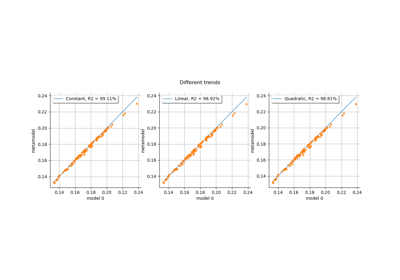
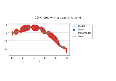
Kriging: choose a polynomial trend on the beam model

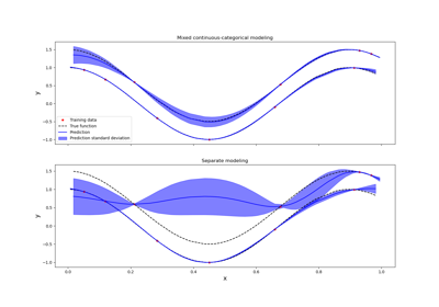
Kriging: metamodel with continuous and categorical variables