GeneralizedParetoFactory
(Source code, png)
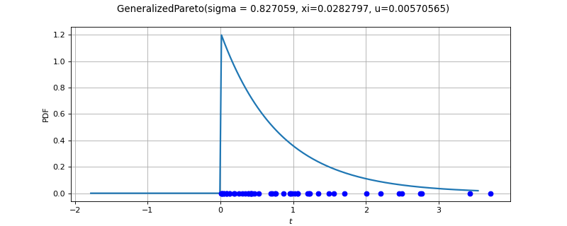
- class GeneralizedParetoFactory(*args)
Generalized Pareto factory.
See also
Notes
The following
ResourceMapentries can be used to tweak the parameters of the optimization solver involved in the different estimators:GeneralizedParetoFactory-DefaultOptimizationAlgorithm
GeneralizedParetoFactory-MaximumEvaluationNumber
GeneralizedParetoFactory-MaximumAbsoluteError
GeneralizedParetoFactory-MaximumRelativeError
GeneralizedParetoFactory-MaximumObjectiveError
GeneralizedParetoFactory-MaximumConstraintError
GeneralizedParetoFactory-InitializationMethod
GeneralizedParetoFactory-NormalizationMethod
Methods
build(*args)Build the distribution.
buildAsGeneralizedPareto(*args)Build the distribution as a GeneralizedPareto type.
buildCovariates(*args)Estimate a GPD from covariates.
buildEstimator(*args)Build the distribution and the parameter distribution.
Build the distribution based on the exponential regression estimator.
buildMethodOfLikelihoodMaximization(sample, u)Estimate the distribution with the maximum likelihood method.
Estimate the distribution and the parameter distribution with the maximum likelihood method.
buildMethodOfMoments(sample)Build the distribution based on the method of moments estimator.
Build the distribution based on the probability weighted moments estimator.
buildMethodOfXiProfileLikelihood(sample, u)Estimate the distribution with the profile likelihood.
Estimate the distribution and the parameter distribution with the profile likelihood.
buildReturnLevelEstimator(result, sample, m)Estimate a return level and its distribution from the GPD parameters.
buildReturnLevelProfileLikelihood(sample, u, m)Estimate a return level and its distribution with the profile likelihood.
Estimate
and its distribution with the profile likelihood.
buildTimeVarying(*args)Estimate a non stationary GPD from a time-dependent parametric model.
drawMeanResidualLife(sample)Draw the mean residual life plot.
drawParameterThresholdStability(sample, ...)Draw the parameter threshold stability plot.
Accessor to the bootstrap size.
Accessor to the object's name.
getName()Accessor to the object's name.
Accessor to the solver.
hasName()Test if the object is named.
setBootstrapSize(bootstrapSize)Accessor to the bootstrap size.
setName(name)Accessor to the object's name.
setOptimizationAlgorithm(solver)Accessor to the solver.
- __init__(*args)
- build(*args)
Build the distribution.
Available usages:
build()
build(sample)
build(param)
- Parameters:
- sample2-d sequence of float, of dimension 1
The sample from which
are estimated.
- paramsequence of float
The parameters of the
GeneralizedPareto.
- Returns:
- dist
Distribution The estimated GPD.
- dist
Notes
In the first usage, the default
GeneralizedParetodistribution is built.In the second usage, the chosen algorithm depends on the size of the sample compared to the
ResourceMapkey GeneralizedParetoFactory-SmallSize (see [matthys2003] for the theory):If the sample size is less or equal to GeneralizedParetoFactory-SmallSize from
ResourceMap, then the method of probability weighted moments is used. If it fails, the method of exponential regression is used.Otherwise, the first method tried is the method of exponential regression, then the method of probability weighted moments if the first one fails.
In the third usage, a
GeneralizedParetodistribution corresponding to the given parameters is built.
- buildAsGeneralizedPareto(*args)
Build the distribution as a GeneralizedPareto type.
Available usages:
build()
build(sample)
build(param)
- Parameters:
- sample2-d sequence of float, of dimension 1
The sample from which
are estimated.
- paramsequence of float,
A vector of parameters of the
GeneralizedPareto.
- Returns:
- dist
GeneralizedPareto The estimated GPD as a
GeneralizedPareto.In the first usage, the default GeneralizedPareto distribution is built.
- dist
Notes
The strategy described in
build()is followed.
- buildCovariates(*args)
Estimate a GPD from covariates.
- Parameters:
- sample2-d sequence of float
Sample drawn from a GPD.
- ufloat
The threshold.
- covariates2-d sequence of float
Covariates sample. A constant column is automatically added if none is not provided.
- sigmaIndicessequence of int, optional
Indices of covariates considered for parameter
.
By default, an empty sequence.
The index of the constant covariate is added if empty or if the covariates do not initially contain a constant column.
- xiIndicessequence of int, optional
Indices of covariates considered for parameter
.
By default, an empty sequence.
The index of the constant covariate is added if empty or if the covariates do not initially contain a constant column.
- sigmaLink
Function, optional The
function.
By default, the identity function.
- xiLink
Function, optional The
function.
By default, the identity function.
- initializationMethodstr, optional
The initialization method for the optimization problem: Generic or Static.
By default, the method Generic (see
ResourceMap, key GeneralizedParetoFactory-InitializationMethod).- normalizationMethodstr, optional
The data normalization method: CenterReduce, MinMax or None.
By default, the method MinMax (see
ResourceMap, key GeneralizedParetoFactory-NormalizationMethod).
- Returns:
- result
CovariatesResult The result class.
- result
Notes
Let
whose excesses above the threshold
follow a GPD whose parameters
depend on
covariates denoted by
:
We assume that the threshold
is known.
We denote by
the values of
associated to the values of the covariates
.
For numerical reasons, it is recommended to normalize the covariates. Each covariate
has its own normalization:
and with three ways of defining
of the covariate
:
the CenterReduce method where
is the covariate mean and
is the standard deviation of the covariates;
the MinMax method where
is the min value of the covariate
and
its range. This is the default method. This is the default method;
the None method where
and
: in that case, data are not normalized.
Let
be the vector of parameters. Then,
depends on all the
covariates even if each component of
only depends on a subset of the covariates. We denote by
the
covariates involved in the modelling of the component
.
Each component
can be written as a function of the normalized covariates:
This relation can be written as a function of the real covariates:
where:
is usually referred to as the inverse-link function of the component
,
each
.
To allow some parameters to remain constant, i.e. independent of the covariates (this will generally be the case for the parameter
), the library systematically adds the constant covariate to the specified covariates.
The complete vector of parameters is defined by:
where
.
The estimator of
maximizes the likelihood of the model which is defined by:
where
denotes the GPD density function with parameters
and evaluated at
.
Then, if none of the
is zero, the log-likelihood is defined by:
defined on
such that
for all
.
And if any of the
is equal to 0, the log-likelihood is defined as:
The initialization of the optimization problem is crucial. Two initial points
are proposed:
the Generic initial point: in that case, we assume that the GPD is stationary and
is the estimate resulting from the method
buildAsGeneralizedPareto()which follows the strategy described in the methodbuild(). This is the default initial point;the Static initial point: in that case, we still assume that the GPD is stationary and
is the maximum likelihood estimate.
The result class provides:
the estimator
,
the asymptotic distribution of
,
the parameter function
,
the graphs of the parameter functions
, where all the components of
are fixed to a reference value excepted for
, for each
,
the graphs of the parameter functions
, where all the components of
are fixed to a reference value excepted for
, for each
,
the normalizing function
,
the optimal log-likelihood value
,
the GEV distribution at covariate
,
the graphs of the quantile functions of order
:
where all the components of
are fixed to a reference value excepted for
, for each
,
the graphs of the quantile functions of order
:
where all the components of
are fixed to a reference value excepted for
, for each
.
- buildEstimator(*args)
Build the distribution and the parameter distribution.
- Parameters:
- sample2-d sequence of float
Data.
- parameters
DistributionParameters Optional, the parametrization.
- Returns:
- resDist
DistributionFactoryResult The results.
- resDist
Notes
According to the way the native parameters of the distribution are estimated, the parameters distribution differs:
Moments method: the asymptotic parameters distribution is normal and estimated by Bootstrap on the initial data;
Maximum likelihood method with a regular model: the asymptotic parameters distribution is normal and its covariance matrix is the inverse Fisher information matrix;
Other methods: the asymptotic parameters distribution is estimated by Bootstrap on the initial data and kernel fitting (see
KernelSmoothing).
If another set of parameters is specified, the native parameters distribution is first estimated and the new distribution is determined from it:
if the native parameters distribution is normal and the transformation regular at the estimated parameters values: the asymptotic parameters distribution is normal and its covariance matrix determined from the inverse Fisher information matrix of the native parameters and the transformation;
in the other cases, the asymptotic parameters distribution is estimated by Bootstrap on the initial data and kernel fitting.
- buildMethodOfExponentialRegression(sample)
Build the distribution based on the exponential regression estimator.
- Parameters:
- sample2-d sequence of float, of dimension 1
The sample from which
are estimated.
- Returns:
- dist
GeneralizedPareto The estimated GPD.
- dist
Notes
Lets denote:
for
Then we estimate
using:
(1)
Where
maximizes:
(2)
under the constraint
.
- buildMethodOfLikelihoodMaximization(sample, u)
Estimate the distribution with the maximum likelihood method.
- Parameters:
- sample2-d sequence of float
Sample drawn from
.
- ufloat
Given threshold value.
- Returns:
- distribution
GeneralizedExtremeValue The estimated distribution of
.
- distribution
Notes
Let
be a random variable whose excesses above
follow a GPD parameterized by
. We assume that
is known.
Let
be a sample drawn from
. We define the excesses above
by:
for all
.
The maximum likelihood estimator of
maximizes the log-likelihood defined by:
If
:
(3)
defined on
such that
for all
.
If
:
(4)
- buildMethodOfLikelihoodMaximizationEstimator(sample, u)
Estimate the distribution and the parameter distribution with the maximum likelihood method.
- Parameters:
- sample2-d sequence of float
Sample drawn from
.
- ufloat
Given threshold value.
- Returns:
- result
DistributionFactoryLikelihoodResult The result class.
- result
Notes
Let
be a random variable whose excesses above
follow a GPD parameterized by
. We assume that
is known.
The estimator
is defined using the profile log-likelihood as detailed in
buildMethodOfLikelihoodMaximization().The result class produced by the method provides:
the GPD distribution associated to
,
the asymptotic distribution of
.
- buildMethodOfMoments(sample)
Build the distribution based on the method of moments estimator.
- Parameters:
- sample2-d sequence of float, of dimension 1
The sample from which
are estimated.
- Returns:
- dist
GeneralizedPareto The estimated GPD.
- dist
Notes
Lets denote:
the empirical mean of the sample,
its empirical variance.
Then, we estimate
using:
(5)
This estimator is well-defined only if
, otherwise the second moment does not exist.
- buildMethodOfProbabilityWeightedMoments(sample)
Build the distribution based on the probability weighted moments estimator.
- Parameters:
- sample2-d sequence of float, of dimension 1
The sample from which
are estimated.
- Returns:
- dist
GeneralizedPareto The estimated GPD.
- dist
Notes
Lets denote:
the sample sorted in ascending order
Then we estimate
using:
(6)
This estimator is well-defined only if
, otherwise the first moment does not exist.
- buildMethodOfXiProfileLikelihood(sample, u)
Estimate the distribution with the profile likelihood.
- Parameters:
- sample2-d sequence of float
Sample drawn from
.
- ufloat
Given threshold value.
- Returns:
- distribution
GeneralizedPareto The estimated GPD.
- distribution
Notes
Let
be a random variable whose excesses above
follow a GPD parameterized by
. We assume that
is known.
The estimator
is defined using a nested numerical optimization of the log-likelihood:
where
is detailed in equations (3) and (4).
The estimator is given by:
- buildMethodOfXiProfileLikelihoodEstimator(sample, u)
Estimate the distribution and the parameter distribution with the profile likelihood.
- Parameters:
- sample2-d sequence of float
Sample drawn from
.
- ufloat
Given threshold value.
- Returns:
- result
ProfileLikelihoodResult The result class.
- result
Notes
Let
be a random variable whose excesses above
follow a GPD parameterized by
. We assume that
is known.
The estimator
is defined in
buildMethodOfXiProfileLikelihood().The result class produced by the method provides:
the GPD distribution associated to
,
the asymptotic distribution of
,
the profile log-likelihood function
,
the optimal profile log-likelihood value
,
confidence intervals of level
of
.
- buildReturnLevelEstimator(result, sample, m, theta=1.0)
Estimate a return level and its distribution from the GPD parameters.
- Parameters:
- result
DistributionFactoryResult Likelihood estimation result obtained to estimate the GPD
.
- sample2-d sequence of float
The initial data from which the clusters (if any) have been extracted. If the data are independent, sample is the sample used to get result.
- mfloat
The return period expressed in terms of number of observations.
- thetafloat, optional
The extremal index defined in (9).
Default value is 1.
- result
- Returns:
- distribution
Distribution The asymptotic distribution of
.
- distribution
Notes
Let
a random variable whose excesses above the threshold
follow a Generalized Pareto distribution
. We assume that
is known.
The
-observation return level
is the level exceeded on average once every
observations. The
-observation return level can be translated into the annual-scale: if there are
observations per year, then the
-year return level corresponds to the
-observation return level where
.
The
-observation return level is defined as a particular quantile of
:
If
:
(7)
If
:
(8)
with
the probability of an exceedance of
and
the extremal index. Denoting the number of observations by
, the number of exceedances of the threshold
by
and the number of clusters obtained above
by
, then
and
are estimated by:
(9)
If the data are independent, no clustering is performed and
.
The estimator
of
is deduced from the estimator
of
of the GPD.
The asymptotic distribution of
is obtained by the Delta method from the asymptotic distribution of
. It is a normal distribution with mean
and variance:
where
and
is the asymptotic covariance of
.
- buildReturnLevelProfileLikelihood(sample, u, m, theta=1.0)
Estimate a return level and its distribution with the profile likelihood.
- Parameters:
- sample2-d sequence of float
A sample of dimension 1.
- ufloat
The threshold.
- mfloat
The return period expressed in terms of number of observations.
- thetafloat, optional
The extremal index defined in (9).
Default value is 1.
- Returns:
- distribution
Normal The asymptotic distribution of
.
- distribution
Notes
Let
a random variable whose excesses above the threshold
follow a Generalized Pareto distribution
. We assume that
is known.
The return level
is defined in
buildReturnLevelEstimator().The estimator
of
is defined using a nested numerical optimization of the log-likelihood:
where
is the log-likelihood detailed in (3) and (4) where we substitued
for
using equations (7) or (8).
Then
is defined by:
The asymptotic distribution of
is normal.
The starting point of the optimization is initialized from the regular maximum likelihood method.
- buildReturnLevelProfileLikelihoodEstimator(sample, u, m, theta=1.0)
Estimate
and its distribution with the profile likelihood.
- Parameters:
- sample2-d sequence of float
A sample of dimension 1.
- ufloat
The threshold.
- mfloat
The return period expressed in terms of number of observations.
- thetafloat, optional
When clustering is performed, this is the ratio
of number of clusters over number of exceedances, otherwise defaults to 1.
- Returns:
- result
ProfileLikelihoodResult The result class.
- result
Notes
Let
a random variable whose excesses above the threshold
follow a Generalized Pareto distribution
. We assume that
is known.
The return level
is defined in
buildReturnLevelEstimator(). The profile log-likelihoodis defined in
buildReturnLevelProfileLikelihood().The result class produced by the method provides:
the GPD distribution associated to
,
the asymptotic distribution of
,
the profile log-likelihood function
,
the optimal profile log-likelihood value
,
confidence intervals of level
of
.
- buildTimeVarying(*args)
Estimate a non stationary GPD from a time-dependent parametric model.
- Parameters:
- sample2-d sequence of float
Sample drawn from
.
- ufloat
The threshold.
- timeStamps2-d sequence of float
Values of
.
- basis
Basis Functional basis.
- sigmaIndicessequence of int, optional
Indices of basis terms considered for parameter
.
- xiIndicessequence of int, optional
Indices of basis terms considered for parameter
.
- sigmaLink
Function, optional The
function.
By default, the identity function.
- xiLink
Function, optional The
function.
By default, the identity function.
- initializationMethodstr, optional
The initialization method for the optimization problem: Generic or Static.
By default, the method Generic (see
ResourceMap, key GeneralizedParetoFactory-InitializationMethod).- normalizationMethodstr, optional
The data normalization method: CenterReduce, MinMax or None.
By default, the method MinMax (see
ResourceMap, key GeneralizedParetoFactory-NormalizationMethod).
- Returns:
- result
TimeVaryingResult The result class.
- result
Notes
Let
be a non stationary random variable whose excesses above the threshold
follow a GPD. We assume that
is known:
We denote by
the values of
on the time stamps
.
For numerical reasons, it is recommended to normalize the time stamps. The following mapping is applied:
and with three ways of defining
:
the CenterReduce method where
is the mean time stamps and
is the standard deviation of the time stamps;
the MinMax method where
is the first time and
the range of the time stamps. This is the default method;
the None method where
and
: in that case, data are not normalized.
If we denote by
is a component of
, then
can be written as a function of
:
where:
is the size of the functional basis involved in the modelling of
,
is usually referred to as the inverse-link function of the parameter
,
each
is a scalar function
,
each
.
We denote by
and
the size of the functional basis of
and
respectively. We denote by
the complete vector of parameters.
The estimator of
maximizes the likelihood of the non stationary model which is defined by:
where
denotes the GPD density function with parameters
evaluated at
.
Then, if none of the
is zero, the log-likelihood is defined by:
defined on
such that
for all
.
And if any of the
is equal to 0, the log-likelihood is defined as:
The initialization of the optimization problem is crucial. Two initial points
are proposed:
the Generic initial point: in that case, we assume that the GPD is stationary and
is the estimate resulting from the method
buildAsGeneralizedPareto()which follows the strategy described in the methodbuild(). This is the default initial point;the Static initial point: in that case, we still assume that the GPD is stationary and
is the maximum likelihood estimate.
The result class produced by the method provides:
the estimator
,
the asymptotic distribution of
,
the parameter functions
,
the normalizing function
,
the optimal log-likelihood value
,
the GPD distribution at time
,
the quantile functions of order
:
.
- drawMeanResidualLife(sample)
Draw the mean residual life plot.
- Parameters:
- sample2-d sequence of float, of dimension 1
The sample drawn from
.
- Returns:
- graph
Graph The graph of
and its
confidence interval.
- graph
Notes
This method is complementary to
drawParameterThresholdStability()as a method of threshold selection.Let
a random variable defined whose excesses above the threshold
follow the Generalized Pareto distribution
. The mean of excesses of
for
is
Hence, for all
is a linear function of
. The threshold
is the smallest value of
from which the curve is linear.
The quantity
is estimated by the empirical estimator of the mean:
The estimator
is asymptotically normal with mean
and variance
.
We denote by
its realization on the sample drawn from
. The mean and the variance of
are respectively estimated by
and
.
The graph
is termed the mean residual life plot.
The confidence level can be set using the
ResourceMapkey GeneralizedParetoFactory-MeanResidualLifeConfidenceLevel The number of threshold points in the graph can be set with the key GeneralizedParetoFactory-MeanResidualLifePointNumber.
- drawParameterThresholdStability(sample, thresholdRange)
Draw the parameter threshold stability plot.
- Parameters:
- sample2-d sequence of float, of dimension 1
The sample drawn from
.
- uRange
Interval The range of the threshold
.
- Returns:
- graph
Graph The graphs of
and
.
- graph
Notes
This method is complementary to
drawMeanResidualLife()as a method of threshold selection.Let
a random variable whose excesses above the threshold
follow a Generalized Pareto distribution
. Then the excesses of
above
also follow a Generalized Pareto distribution
where:
(10)
Hence, if we define the modified scale parameter
by:
then , by virtue of (10),
is constant with respect to
.
Consequently, estimates of
and
should be constant (or stable accounting for sampling variability) above
if
is a valid threshold for excesses to follow a Generalized Pareto distribution.
The method draws the graphs of
and
with the respective
confidence intervals, for
. The selected threshold is the lowest value of
from which the estimates remain near-constant.
The confidence level can be set using the
ResourceMapkey GeneralizedParetoFactory-ThresholdStabilityConfidenceLevel The number of threshold points in the graph can be set with the key GeneralizedParetoFactory-ThresholdStabilityPointNumber.
- getBootstrapSize()
Accessor to the bootstrap size.
- Returns:
- sizeint
Size of the bootstrap.
- getClassName()
Accessor to the object’s name.
- Returns:
- class_namestr
The object class name (object.__class__.__name__).
- getName()
Accessor to the object’s name.
- Returns:
- namestr
The name of the object.
- getOptimizationAlgorithm()
Accessor to the solver.
- Returns:
- solver
OptimizationAlgorithm The solver used for numerical optimization of the likelihood.
- solver
- hasName()
Test if the object is named.
- Returns:
- hasNamebool
True if the name is not empty.
- setBootstrapSize(bootstrapSize)
Accessor to the bootstrap size.
- Parameters:
- sizeint
The size of the bootstrap.
- setName(name)
Accessor to the object’s name.
- Parameters:
- namestr
The name of the object.
- setOptimizationAlgorithm(solver)
Accessor to the solver.
- Parameters:
- solver
OptimizationAlgorithm The solver used for numerical optimization of the likelihood.
- solver
 OpenTURNS
