FixedStrategy
- class FixedStrategy(*args)
Fixed truncation strategy.
- Parameters:
- orthogonalBasis
OrthogonalBasis An OrthogonalBasis.
- dimensionpositive int
Number of terms of the basis.
- orthogonalBasis
Methods
Compute initial basis for the approximation.
getBasis()Accessor to the underlying orthogonal basis.
Accessor to the object's name.
Accessor to the maximum dimension of the orthogonal basis.
getName()Accessor to the object's name.
getPsi()Accessor to the selected orthogonal polynomials in the basis.
hasName()Test if the object is named.
Get the model selection flag.
setMaximumDimension(maximumDimension)Accessor to the maximum dimension of the orthogonal basis.
setName(name)Accessor to the object's name.
updateBasis(alpha_k, residual, relativeError)Update the basis for the next iteration of approximation.
See also
Notes
The so-called fixed strategy simply consists in selecting the first
 elements of the PC basis, the latter being ordered according to a given
EnumerateFunction(hyperbolic or not). The retained set is built in a single pass. The truncated PC expansion is given by:
In case of a
LinearEnumerateFunction, for a given natural integer representing the total polynomial degree, the number of
coefficients is equal to:
representing the total polynomial degree, the number of
coefficients is equal to:
where
 is the input dimension.
This way the set of retained basis functions
is the input dimension.
This way the set of retained basis functions  gathers all the polynomials with total degree not greater than .
The number of terms grows polynomially both in and
though, which may lead to difficulties in terms of computational efficiency and
memory requirements when dealing with high-dimensional problems.
gathers all the polynomials with total degree not greater than .
The number of terms grows polynomially both in and
though, which may lead to difficulties in terms of computational efficiency and
memory requirements when dealing with high-dimensional problems.Examples
>>> import openturns as ot
>>> ot.RandomGenerator.SetSeed(0)
>>> # Define the model
>>> inputDim = 1
>>> model = ot.SymbolicFunction(['x'], ['x*sin(x)'])
>>> # Create the input distribution
>>> distribution = ot.JointDistribution([ot.Uniform()]*inputDim)
>>> # Construction of the multivariate orthonormal basis
>>> polyColl = [0.0]*inputDim
>>> for i in range(distribution.getDimension()):
...     polyColl[i] = ot.StandardDistributionPolynomialFactory(distribution.getMarginal(i))
>>> enumerateFunction = ot.LinearEnumerateFunction(inputDim)
>>> productBasis = ot.OrthogonalProductPolynomialFactory(polyColl, enumerateFunction)
>>> # Truncature strategy of the multivariate orthonormal basis
>>> # We choose all the polynomials of degree <= 4
>>> degree = 4
>>> indexMax = enumerateFunction.getStrataCumulatedCardinal(degree)
>>> print(indexMax)
5
>>> # We keep all the polynomials of degree <= 4
>>> # which corresponds to the 5 first ones
>>> adaptiveStrategy = ot.FixedStrategy(productBasis, indexMax)
- __init__(*args)
- getBasis()
Accessor to the underlying orthogonal basis.
- Returns:
- basis
OrthogonalBasis Orthogonal basis of which the adaptive strategy is based.
- basis
- getClassName()
Accessor to the object’s name.
- Returns:
- class_namestr
The object class name (object.__class__.__name__).
- getMaximumDimension()
Accessor to the maximum dimension of the orthogonal basis.
- Returns:
- maximumDimensionint
Maximum dimension of the truncated basis.
- getName()
Accessor to the object’s name.
- Returns:
- namestr
The name of the object.
- getPsi()
Accessor to the selected orthogonal polynomials in the basis.
The value returned by this method depends on the specific choice of adaptive strategy and the previous calls to the
updateBasis()method.- Returns:
- polynomialslist of polynomials
Sequence of
polynomials.
Notes
The method
computeInitialBasis()must be applied first.Examples
>>> import openturns as ot
>>> productBasis = ot.OrthogonalProductPolynomialFactory([ot.HermiteFactory()])
>>> adaptiveStrategy = ot.FixedStrategy(productBasis, 3)
>>> adaptiveStrategy.computeInitialBasis()
>>> print(adaptiveStrategy.getPsi())
[1,x0,-0.707107 + 0.707107 * x0^2]
- hasName()
Test if the object is named.
- Returns:
- hasNamebool
True if the name is not empty.
- involvesModelSelection()
Get the model selection flag.
A model selection method can be used to select the coefficients of the decomposition which enable to best predict the output. Model selection can lead to a sparse functional chaos expansion.
- Returns:
- involvesModelSelectionbool
True if the method involves a model selection method.
- setMaximumDimension(maximumDimension)
Accessor to the maximum dimension of the orthogonal basis.
- Parameters:
- maximumDimensionint
Maximum dimension of the truncated basis.
- setName(name)
Accessor to the object’s name.
- Parameters:
- namestr
The name of the object.
- updateBasis(alpha_k, residual, relativeError)
Update the basis for the next iteration of approximation.
No changes are made to the basis in the fixed strategy. Hence, the number of functions in the basis is equal to dimension, whatever the number of calls to the updateBasis method.
- Parameters:
- alpha_ksequence of floats
The coefficients of the expansion at this step.
- residualfloat
The current value of the residual.
- relativeErrorfloat
The relative error.
Examples using the class


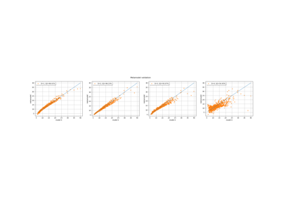
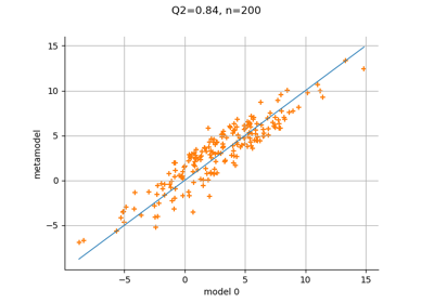
Create a full or sparse polynomial chaos expansion
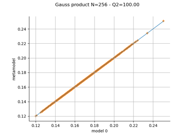
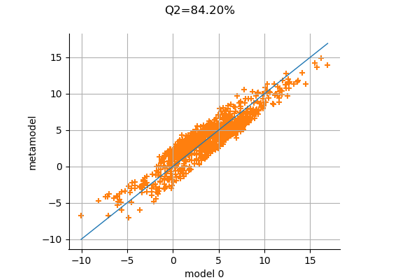
Create a polynomial chaos metamodel by integration on the cantilever beam

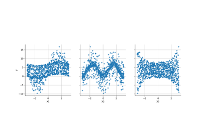
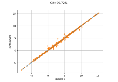
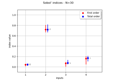
Create a polynomial chaos for the Ishigami function: a quick start guide to polynomial chaos
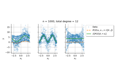
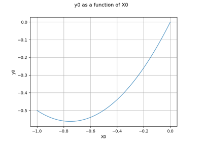
Conditional expectation of a polynomial chaos expansion
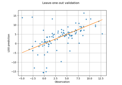
Compute leave-one-out error of a polynomial chaos expansion