LeastSquaresStrategy
- class LeastSquaresStrategy(*args)
Least squares strategy for the approximation coefficients.
- Available constructors:
LeastSquaresStrategy(weightedExp)
LeastSquaresStrategy(weightedExp, approxAlgoImpFact)
LeastSquaresStrategy(approxAlgoImpFact)
LeastSquaresStrategy(measure, approxAlgoImpFact)
LeastSquaresStrategy(measure, weightedExp, approxAlgoImpFact)
LeastSquaresStrategy(inputSample, outputSample, approxAlgoImpFact)
LeastSquaresStrategy(inputSample, weights, outputSample, approxAlgoImpFact)
- Parameters:
- weightedExp
WeightedExperiment Experimental design used for the transformed input data. By default the class
MonteCarloExperimentis used.- approxAlgoImpFactApproximationAlgorithmImplementationFactory
The factory that builds the desired
ApproximationAlgorithm. By default the classPenalizedLeastSquaresAlgorithmFactoryis used.- measure
Distribution Distribution
 with respect to which the basis is orthonormal.
By default, the limit measure defined within the class
with respect to which the basis is orthonormal.
By default, the limit measure defined within the class
WeightedExperimentis used.- inputSample2-d sequence of float
The input random observations
 where
where  is the input of the physical
model,
is the input of the physical
model,  is the input dimension and
  is the sample size.
- outputSample2-d sequence of float
The output random observations
 where
where  is the output of the physical
model,
is the output of the physical
model,  is the output dimension and is the sample size.
- weightssequence of float
Numerical point that are the weights associated to the input sample points such that the corresponding weighted experiment is a good approximation of
. If not precised, all weights are equals to
 , where is the size of the
sample.
, where is the size of the
sample.
- weightedExp
Methods
Accessor to the object's name.
Accessor to the coefficients.
Accessor to the design proxy.
Accessor to the experiments.
Accessor to the input sample.
Accessor to the measure.
getName()Accessor to the object's name.
Accessor to the output sample.
Accessor to the relative error.
Accessor to the residual.
Accessor to the weights.
hasName()Test if the object is named.
Get the model selection flag.
Get the least squares flag.
setExperiment(weightedExperiment)Accessor to the design of experiment.
setInputSample(inputSample)Accessor to the input sample.
setMeasure(measure)Accessor to the measure.
setName(name)Accessor to the object's name.
setOutputSample(outputSample)Accessor to the output sample.
setWeights(weights)Accessor to the weights.
Notes
This class is not usable because it has sense only within the
FunctionalChaosAlgorithm: the least squares strategy evaluates the coefficients of the polynomials
decomposition as follows:
of the polynomials
decomposition as follows:![\vect{a} = \argmin_{\vect{b} \in \Rset^P} E_{\mu} \left[ \left( g \circ T^{-1}
(\vect{U}) - \vect{b}^{\intercal} \vect{\Psi}(\vect{U}) \right)^2 \right]](data:image/svg+xml;base64,PD94bWwgdmVyc2lvbj0nMS4wJyBlbmNvZGluZz0nVVRGLTgnPz4KPCEtLSBUaGlzIGZpbGUgd2FzIGdlbmVyYXRlZCBieSBkdmlzdmdtIDMuNC4yIC0tPgo8c3ZnIHZlcnNpb249JzEuMScgeG1sbnM9J2h0dHA6Ly93d3cudzMub3JnLzIwMDAvc3ZnJyB4bWxuczp4bGluaz0naHR0cDovL3d3dy53My5vcmcvMTk5OS94bGluaycgd2lkdGg9JzIxNy43MzczNDhwdCcgaGVpZ2h0PScyNC45MjI3MzdwdCcgdmlld0JveD0nODUuNDAyODA4IC0yNi4xMTgyNTEgMjE3LjczNzM0OCAyNC45MjI3MzcnPgo8ZGVmcz4KPHBhdGggaWQ9J2cyLTknIGQ9J001LjkwNTg1My03LjY4NzE3M0g3LjQ5NTg5Vi04LjIwMTI0NUM2Ljk5Mzc3My04LjE3NzMzNSA1LjczODQ4MS04LjE3NzMzNSA1LjE3NjU4OC04LjE3NzMzNVMzLjM0NzQ0Ny04LjE3NzMzNSAyLjg0NTMzLTguMjAxMjQ1Vi03LjY4NzE3M0g0LjQzNTM2N1YtMi4yNDc1NzJDMy4zNTk0MDItMi41ODIzMTYgMi45ODg3OTItMy40NTUwNDQgMi45NzY4MzctNC45NjEzOTVDMi45NjQ4ODItNi4xNTY5MTIgMi41ODIzMTYtNi41NzUzNDIgMS45MjQ3ODItNi41NzUzNDJIMS4wODc5MkMuOTA4NTkzLTYuNTc1MzQyIC43NDEyMi02LjU3NTM0MiAuNzQxMjItNi4zNzIxMDVDLjc0MTIyLTYuMjg4NDE4IC43ODkwNDEtNi4yMDQ3MzIgLjg5NjYzOC02LjE4MDgyMkMxLjA2NDAxLTYuMTU2OTEyIDEuMjMxMzgyLTYuMTQ0OTU2IDEuMzUwOTM0LTUuODY5OTg4QzEuNDk0Mzk2LTUuNTM1MjQzIDEuNTA2MzUxLTUuMDgwOTQ2IDEuNTA2MzUxLTUuMDU3MDM2QzEuNTA2MzUxLTQuNTU0OTE5IDEuNTE4MzA2LTMuNTUwNjg1IDIuMjIzNjYxLTIuNzYxNjQ0QzIuOTQwOTcxLTEuOTQ4NjkyIDQuMDI4ODkyLTEuODI5MTQxIDQuNDM1MzY3LTEuNzgxMzJWLS41MTQwNzJIMi44NDUzM1YwQzMuMzQ3NDQ3LS4wMjM5MSA0LjYwMjc0LS4wMjM5MSA1LjE2NDYzMy0uMDIzOTFTNi45OTM3NzMtLjAyMzkxIDcuNDk1ODkgMFYtLjUxNDA3Mkg1LjkwNTg1M1YtMS43ODEzMkM2Ljc3ODU4LTEuODUzMDUxIDcuNjAzNDg3LTIuMTE2MDY1IDguMjEzMi0yLjc2MTY0NFM4Ljk0MjQ2Ni00LjM5OTUwMiA4Ljk0MjQ2Ni00LjczNDI0N0M4Ljk0MjQ2Ni01LjIxMjQ1MyA4Ljk1NDQyMS02LjEwOTA5MSA5LjQ2ODQ5My02LjE4MDgyMkM5LjYtNi4xOTI3NzcgOS43MDc1OTctNi4yMTY2ODcgOS43MDc1OTctNi4zNzIxMDVDOS43MDc1OTctNi41NzUzNDIgOS41NjQxMzQtNi41NzUzNDIgOS4zNjA4OTctNi41NzUzNDJIOC41MjQwMzVDNy42OTkxMjgtNi41NzUzNDIgNy40ODM5MzUtNS45Mjk3NjMgNy40NzE5OC00Ljg0MTg0M0M3LjQ2MDAyNS0zLjQzMTEzMyA3LjAwNTcyOS0yLjUxMDU4NSA1LjkwNTg1My0yLjIzNTYxNlYtNy42ODcxNzNaJy8+CjxwYXRoIGlkPSdnNC0xMjQnIGQ9J00yLjUzNDQ5Ni0yLjc5NzUwOUgzLjU2MjY0QzMuNjc0MjIyLTIuNzk3NTA5IDMuOTg1MDU2LTIuNzk3NTA5IDMuOTg1MDU2LTMuMTE2MzE0UzMuNjc0MjIyLTMuNDM1MTE4IDMuNTYyNjQtMy40MzUxMThILjg2ODc0MkMuNzU3MTYxLTMuNDM1MTE4IC40NDYzMjYtMy40MzUxMTggLjQ0NjMyNi0zLjExNjMxNFMuNzU3MTYxLTIuNzk3NTA5IC44Njg3NDItMi43OTc1MDlIMS44OTY4ODdWMS4yNzUyMThDMS44OTY4ODcgMS4zODY4IDEuODk2ODg3IDEuNjk3NjM0IDIuMjE1NjkxIDEuNjk3NjM0UzIuNTM0NDk2IDEuMzg2OCAyLjUzNDQ5NiAxLjI3NTIxOFYtMi43OTc1MDlaJy8+CjxwYXRoIGlkPSdnMTEtNDknIGQ9J00yLjUwMjYxNS01LjA3Njk2MUMyLjUwMjYxNS01LjI5MjE1NCAyLjQ4NjY3NS01LjMwMDEyNSAyLjI3MTQ4Mi01LjMwMDEyNUMxLjk0NDcwNy00Ljk4MTMyIDEuNTIyMjkxLTQuNzkwMDM3IC43NjUxMzEtNC43OTAwMzdWLTQuNTI3MDI0Qy45ODAzMjQtNC41MjcwMjQgMS40MTA3MS00LjUyNzAyNCAxLjg3Mjk3Ni00Ljc0MjIxN1YtLjY1MzU0OUMxLjg3Mjk3Ni0uMzU4NjU1IDEuODQ5MDY2LS4yNjMwMTQgMS4wOTE5MDUtLjI2MzAxNEguODEyOTUxVjBDMS4xMzk3MjYtLjAyMzkxIDEuODI1MTU2LS4wMjM5MSAyLjE4MzgxMS0uMDIzOTFTMy4yMzU4NjYtLjAyMzkxIDMuNTYyNjQgMFYtLjI2MzAxNEgzLjI4MzY4NkMyLjUyNjUyNi0uMjYzMDE0IDIuNTAyNjE1LS4zNTg2NTUgMi41MDI2MTUtLjY1MzU0OVYtNS4wNzY5NjFaJy8+CjxwYXRoIGlkPSdnMTEtNTAnIGQ9J00yLjI0NzU3Mi0xLjYyNTkwM0MyLjM3NTA5My0xLjc0NTQ1NSAyLjcwOTgzOC0yLjAwODQ2OCAyLjgzNzM2LTIuMTIwMDVDMy4zMzE1MDctMi41NzQzNDYgMy44MDE3NDMtMy4wMTI3MDIgMy44MDE3NDMtMy43Mzc5ODNDMy44MDE3NDMtNC42ODY0MjYgMy4wMDQ3MzItNS4zMDAxMjUgMi4wMDg0NjgtNS4zMDAxMjVDMS4wNTIwNTUtNS4zMDAxMjUgLjQyMjQxNi00LjU3NDg0NCAuNDIyNDE2LTMuODY1NTA0Qy40MjI0MTYtMy40NzQ5NjkgLjczMzI1LTMuNDE5MTc4IC44NDQ4MzItMy40MTkxNzhDMS4wMTIyMDQtMy40MTkxNzggMS4yNTkyNzgtMy41Mzg3MyAxLjI1OTI3OC0zLjg0MTU5NEMxLjI1OTI3OC00LjI1NjA0IC44NjA3NzItNC4yNTYwNCAuNzY1MTMxLTQuMjU2MDRDLjk5NjI2NC00LjgzNzg1OCAxLjUzMDI2Mi01LjAzNzExMSAxLjkyMDc5Ny01LjAzNzExMUMyLjY2MjAxNy01LjAzNzExMSAzLjA0NDU4My00LjQwNzQ3MiAzLjA0NDU4My0zLjczNzk4M0MzLjA0NDU4My0yLjkwOTA5MSAyLjQ2Mjc2NS0yLjMwMzM2MiAxLjUyMjI5MS0xLjMzODk3OUwuNTE4MDU3LS4zMDI4NjRDLjQyMjQxNi0uMjE1MTkzIC40MjI0MTYtLjE5OTI1MyAuNDIyNDE2IDBIMy41NzA2MUwzLjgwMTc0My0xLjQyNjY1SDMuNTU0NjdDMy41MzA3Ni0xLjI2NzI0OCAzLjQ2Njk5OS0uODY4NzQyIDMuMzcxMzU3LS43MTczMUMzLjMyMzUzNy0uNjUzNTQ5IDIuNzE3ODA4LS42NTM1NDkgMi41OTAyODYtLjY1MzU0OUgxLjE3MTYwNkwyLjI0NzU3Mi0xLjYyNTkwM1onLz4KPHBhdGggaWQ9J2c3LTAnIGQ9J003Ljg3ODQ1Ni0yLjc0OTY4OUM4LjA4MTY5NC0yLjc0OTY4OSA4LjI5Njg4Ny0yLjc0OTY4OSA4LjI5Njg4Ny0yLjk4ODc5MlM4LjA4MTY5NC0zLjIyNzg5NSA3Ljg3ODQ1Ni0zLjIyNzg5NUgxLjQxMDcxQzEuMjA3NDcyLTMuMjI3ODk1IC45OTIyNzktMy4yMjc4OTUgLjk5MjI3OS0yLjk4ODc5MlMxLjIwNzQ3Mi0yLjc0OTY4OSAxLjQxMDcxLTIuNzQ5Njg5SDcuODc4NDU2WicvPgo8cGF0aCBpZD0nZzctMTQnIGQ9J001LjMwODA5NS0yLjk4ODc5MkM1LjMwODA5NS00LjI2Nzk5NSA0LjI0NDA4NS01LjMwODA5NSAyLjk4ODc5Mi01LjMwODA5NUMxLjY5NzYzNC01LjMwODA5NSAuNjU3NTM0LTQuMjQ0MDg1IC42NTc1MzQtMi45ODg3OTJDLjY1NzUzNC0xLjcyMTU0NCAxLjY5NzYzNC0uNjY5NDg5IDIuOTg4NzkyLS42Njk0ODlDNC4yNDQwODUtLjY2OTQ4OSA1LjMwODA5NS0xLjcwOTU4OSA1LjMwODA5NS0yLjk4ODc5MlpNMi45ODg3OTItMS4xNDc2OTZDMS45NDg2OTItMS4xNDc2OTYgMS4xMzU3NDEtMS45ODQ1NTggMS4xMzU3NDEtMi45ODg3OTJTMS45NjA2NDgtNC44Mjk4ODggMi45ODg3OTItNC44Mjk4ODhDMy45ODEwNzEtNC44Mjk4ODggNC44Mjk4ODgtNC4wMTY5MzYgNC44Mjk4ODgtMi45ODg3OTJTMy45ODEwNzEtMS4xNDc2OTYgMi45ODg3OTItMS4xNDc2OTZaJy8+CjxwYXRoIGlkPSdnOS0yMicgZD0nTTEuOTI4NzY3LTIuODEzNDVDMS45Njg2MTgtMi45NjQ4ODIgMi4wMzIzNzktMy4yMjc4OTUgMi4wMzIzNzktMy4yNjc3NDZDMi4wMzIzNzktMy40MzUxMTggMS45MDQ4NTctMy41MTQ4MTkgMS43NjkzNjUtMy41MTQ4MTlDMS40OTgzODEtMy41MTQ4MTkgMS40MzQ2Mi0zLjI1MTgwNiAxLjQwMjc0LTMuMTQwMjI0TC4yOTQ4OTQgMS4yODMxODhDLjI2MzAxNCAxLjQxMDcxIC4yNjMwMTQgMS40NTA1NiAuMjYzMDE0IDEuNDY2NTAxQy4yNjMwMTQgMS42NjU3NTMgLjQyMjQxNiAxLjcxMzU3NCAuNTE4MDU3IDEuNzEzNTc0Qy41NTc5MDggMS43MTM1NzQgLjc0MTIyIDEuNzA1NjA0IC44NDQ4MzIgMS40OTgzODFDLjg2ODc0MiAxLjQzNDYyIDEuMDk5ODc1IC40ODYxNzcgMS4yNTkyNzgtLjE1MTQzMkMxLjM5NDc3LS4wNDc4MjEgMS42NjU3NTMgLjA3OTcwMSAyLjA3MjIyOSAuMDc5NzAxQzIuNzI1Nzc4IC4wNzk3MDEgMy4xNTYxNjQtLjQ1NDI5NiAzLjE4MDA3NS0uNDg2MTc3QzMuMzIzNTM3IC4wNjM3NjEgMy44NjU1MDQgLjA3OTcwMSAzLjk2MTE0NiAuMDc5NzAxQzQuMzI3NzcxIC4wNzk3MDEgNC41MTEwODMtLjIyMzE2MyA0LjU3NDg0NC0uMzU4NjU1QzQuNzM0MjQ3LS42NDU1NzkgNC44NDU4MjgtMS4xMDc4NDYgNC44NDU4MjgtMS4xMzk3MjZDNC44NDU4MjgtMS4xODc1NDcgNC44MTM5NDgtMS4yNDMzMzcgNC43MTgzMDYtMS4yNDMzMzdTNC42MDY3MjUtMS4xOTU1MTcgNC41NTg5MDQtLjk5NjI2NEM0LjQ0NzMyMy0uNTU3OTA4IDQuMjk1ODktLjE0MzQ2MiAzLjk4NTA1Ni0uMTQzNDYyQzMuODAxNzQzLS4xNDM0NjIgMy43MzAwMTItLjI5NDg5NCAzLjczMDAxMi0uNTE4MDU3QzMuNzMwMDEyLS42NTM1NDkgMy44MTc2ODQtLjk5NjI2NCAzLjg3MzQ3NC0xLjIyNzM5N0w0LjA4MDY5Ny0yLjA0MDM0OUM0LjEyODUxOC0yLjI0NzU3MiA0LjE2ODM2OS0yLjQxNDk0NCA0LjIzMjEzLTIuNjU0MDQ3QzQuMjcxOTgtMi44MjkzOSA0LjM1MTY4MS0zLjE0MDIyNCA0LjM1MTY4MS0zLjE4ODA0NUM0LjM1MTY4MS0zLjM4NzI5OCA0LjE5MjI3OS0zLjQzNTExOCA0LjA5NjYzOC0zLjQzNTExOEMzLjgxNzY4NC0zLjQzNTExOCAzLjc2OTg2My0zLjIzNTg2NiAzLjY4MjE5Mi0yLjg3NzIxTDMuNTE0ODE5LTIuMjE1NjkxTDMuMjY3NzQ2LTEuMjE5NDI3TDMuMTg4MDQ1LS45MDA2MjNDMy4xNzIxMDUtLjg1MjgwMiAyLjk1NjkxMi0uNTQ5OTM4IDIuNzczNTk5LS4zOTg1MDZDMi42MzgxMDctLjI5NDg5NCAyLjQwNjk3NC0uMTQzNDYyIDIuMTEyMDgtLjE0MzQ2MkMxLjczNzQ4NC0uMTQzNDYyIDEuNDgyNDQxLS4zNDI3MTUgMS40ODI0NDEtLjgzNjg2MkMxLjQ4MjQ0MS0xLjA0NDA4NSAxLjU0NjIwMi0xLjI4MzE4OCAxLjU5NDAyMi0xLjQ3NDQ3MUwxLjkyODc2Ny0yLjgxMzQ1WicvPgo8cGF0aCBpZD0nZzEwLTY5JyBkPSdNOC4zMDg4NDItMi43NzM1OTlDOC4zMjA3OTctMi44MDk0NjUgOC4zNTY2NjMtMi44OTMxNTEgOC4zNTY2NjMtMi45NDA5NzFDOC4zNTY2NjMtMy4wMDA3NDcgOC4zMDg4NDItMy4wNjA1MjMgOC4yMzcxMTEtMy4wNjA1MjNDOC4xODkyOS0zLjA2MDUyMyA4LjE2NTM4LTMuMDQ4NTY4IDguMTI5NTE0LTMuMDEyNzAyQzguMTA1NjA0LTMuMDAwNzQ3IDguMTA1NjA0LTIuOTc2ODM3IDcuOTk4MDA3LTIuNzM3NzMzQzcuMjkyNjUzLTEuMDY0MDEgNi43Nzg1OC0uMzQ2NyA0Ljg2NTc1My0uMzQ2N0gzLjEyMDI5OUMyLjk1MjkyNy0uMzQ2NyAyLjkyOTAxNi0uMzQ2NyAyLjg1NzI4NS0uMzU4NjU1QzIuNzI1Nzc4LS4zNzA2MSAyLjcxMzgyMy0uMzk0NTIxIDIuNzEzODIzLS40OTAxNjJDMi43MTM4MjMtLjU3Mzg0OCAyLjczNzczMy0uNjQ1NTc5IDIuNzYxNjQ0LS43NTMxNzZMMy41ODY1NS00LjA1MjgwMkg0Ljc3MDExMkM1LjcwMjYxNS00LjA1MjgwMiA1Ljc3NDM0Ni0zLjg0OTU2NCA1Ljc3NDM0Ni0zLjQ5MDkwOUM1Ljc3NDM0Ni0zLjM3MTM1NyA1Ljc3NDM0Ni0zLjI2Mzc2MSA1LjY5MDY2LTIuOTA1MTA2QzUuNjY2NzUtMi44NTcyODUgNS42NTQ3OTUtMi44MDk0NjUgNS42NTQ3OTUtMi43NzM1OTlDNS42NTQ3OTUtMi42ODk5MTMgNS43MTQ1Ny0yLjY1NDA0NyA1Ljc4NjMwMS0yLjY1NDA0N0M1Ljg5Mzg5OC0yLjY1NDA0NyA1LjkwNTg1My0yLjczNzczMyA1Ljk1MzY3NC0yLjkwNTEwNkw2LjYzNTExOC01LjY3ODcwNUM2LjYzNTExOC01LjczODQ4MSA2LjU4NzI5OC01Ljc5ODI1NyA2LjUxNTU2Ny01Ljc5ODI1N0M2LjQwNzk3LTUuNzk4MjU3IDYuMzk2MDE1LTUuNzUwNDM2IDYuMzQ4MTk0LTUuNTgzMDY0QzYuMTA5MDkxLTQuNjYyNTE2IDUuODY5OTg4LTQuMzk5NTAyIDQuODA1OTc4LTQuMzk5NTAySDMuNjcwMjM3TDQuNDExNDU3LTcuMzQwNDczQzQuNTE5MDU0LTcuNzU4OTA0IDQuNTQyOTY0LTcuNzk0NzcgNS4wMzMxMjYtNy43OTQ3N0g2Ljc0MjcxNUM4LjIxMzItNy43OTQ3NyA4LjUxMjA4LTcuNDAwMjQ5IDguNTEyMDgtNi40OTE2NTZDOC41MTIwOC02LjQ3OTcwMSA4LjUxMjA4LTYuMTQ0OTU2IDguNDY0MjU5LTUuNzUwNDM2QzguNDUyMzA0LTUuNzAyNjE1IDguNDQwMzQ5LTUuNjMwODg0IDguNDQwMzQ5LTUuNjA2OTc0QzguNDQwMzQ5LTUuNTExMzMzIDguNTAwMTI1LTUuNDc1NDY3IDguNTcxODU2LTUuNDc1NDY3QzguNjU1NTQyLTUuNDc1NDY3IDguNzAzMzYyLTUuNTIzMjg4IDguNzI3MjczLTUuNzM4NDgxTDguOTc4MzMxLTcuODMwNjM1QzguOTc4MzMxLTcuODY2NTAxIDkuMDAyMjQyLTcuOTg2MDUyIDkuMDAyMjQyLTguMDA5OTYzQzkuMDAyMjQyLTguMTQxNDY5IDguODk0NjQ1LTguMTQxNDY5IDguNjc5NDUyLTguMTQxNDY5SDIuODQ1MzNDMi42MTgxODItOC4xNDE0NjkgMi40OTg2My04LjE0MTQ2OSAyLjQ5ODYzLTcuOTI2Mjc2QzIuNDk4NjMtNy43OTQ3NyAyLjU4MjMxNi03Ljc5NDc3IDIuNzg1NTU0LTcuNzk0NzdDMy41MjY3NzUtNy43OTQ3NyAzLjUyNjc3NS03LjcxMTA4MyAzLjUyNjc3NS03LjU3OTU3N0MzLjUyNjc3NS03LjUxOTgwMSAzLjUxNDgxOS03LjQ3MTk4IDMuNDc4OTU0LTcuMzQwNDczTDEuODY1MDA2LS44ODQ2ODJDMS43NTc0MS0uNDY2MjUyIDEuNzMzNDk5LS4zNDY3IC44OTY2MzgtLjM0NjdDLjY2OTQ4OS0uMzQ2NyAuNTQ5OTM4LS4zNDY3IC41NDk5MzgtLjEzMTUwN0MuNTQ5OTM4IDAgLjYyMTY2OSAwIC44NjA3NzIgMEg2Ljg2MjI2N0M3LjEyNTI4IDAgNy4xMzcyMzUtLjAxMTk1NSA3LjIyMDkyMi0uMjAzMjM4TDguMzA4ODQyLTIuNzczNTk5WicvPgo8cGF0aCBpZD0nZzEwLTg0JyBkPSdNNC45ODUzMDUtNy4yOTI2NTNDNS4wNTcwMzYtNy41Nzk1NzcgNS4wODA5NDYtNy42ODcxNzMgNS4yNjAyNzQtNy43MzQ5OTRDNS4zNTU5MTUtNy43NTg5MDQgNS43NTA0MzYtNy43NTg5MDQgNi4wMDE0OTQtNy43NTg5MDRDNy4xOTcwMTEtNy43NTg5MDQgNy43NTg5MDQtNy43MTEwODMgNy43NTg5MDQtNi43Nzg1OEM3Ljc1ODkwNC02LjU5OTI1MyA3LjcxMTA4My02LjE0NDk1NiA3LjYzOTM1Mi01LjcwMjYxNUw3LjYyNzM5Ny01LjU1OTE1M0M3LjYyNzM5Ny01LjUxMTMzMyA3LjY3NTIxOC01LjQzOTYwMSA3Ljc0Njk0OS01LjQzOTYwMUM3Ljg2NjUwMS01LjQzOTYwMSA3Ljg2NjUwMS01LjQ5OTM3NyA3LjkwMjM2Ni01LjY5MDY2TDguMjQ5MDY2LTcuODA2NzI1QzguMjcyOTc2LTcuOTE0MzIxIDguMjcyOTc2LTcuOTM4MjMyIDguMjcyOTc2LTcuOTc0MDk3QzguMjcyOTc2LTguMTA1NjA0IDguMjAxMjQ1LTguMTA1NjA0IDcuOTYyMTQyLTguMTA1NjA0SDEuNDIyNjY1QzEuMTQ3Njk2LTguMTA1NjA0IDEuMTM1NzQxLTguMDkzNjQ5IDEuMDY0MDEtNy44Nzg0NTZMLjMzNDc0NS01LjcyNjUyNkMuMzIyNzktNS43MDI2MTUgLjI4NjkyNC01LjU3MTEwOCAuMjg2OTI0LTUuNTU5MTUzQy4yODY5MjQtNS40OTkzNzcgLjMzNDc0NS01LjQzOTYwMSAuNDA2NDc2LTUuNDM5NjAxQy41MDIxMTctNS40Mzk2MDEgLjUyNjAyNy01LjQ4NzQyMiAuNTczODQ4LTUuNjQyODM5QzEuMDc1OTY1LTcuMDg5NDE1IDEuMzI3MDI0LTcuNzU4OTA0IDIuOTE3MDYxLTcuNzU4OTA0SDMuNzE4MDU3QzQuMDA0OTgxLTcuNzU4OTA0IDQuMTI0NTMzLTcuNzU4OTA0IDQuMTI0NTMzLTcuNjI3Mzk3QzQuMTI0NTMzLTcuNTkxNTMyIDQuMTI0NTMzLTcuNTY3NjIxIDQuMDY0NzU3LTcuMzUyNDI4TDIuNDYyNzY1LS45MzI1MDNDMi4zNDMyMTMtLjQ2NjI1MiAyLjMxOTMwMy0uMzQ2NyAxLjA1MjA1NS0uMzQ2N0MuNzUzMTc2LS4zNDY3IC42Njk0ODktLjM0NjcgLjY2OTQ4OS0uMTE5NTUyQy42Njk0ODkgMCAuODAwOTk2IDAgLjg2MDc3MiAwQzEuMTU5NjUxIDAgMS40NzA0ODYtLjAyMzkxIDEuNzY5MzY1LS4wMjM5MUgzLjYzNDM3MUMzLjkzMzI1LS4wMjM5MSA0LjI1NjA0IDAgNC41NTQ5MTkgMEM0LjY4NjQyNiAwIDQuODA1OTc4IDAgNC44MDU5NzgtLjIyNzE0OEM0LjgwNTk3OC0uMzQ2NyA0LjcyMjI5MS0uMzQ2NyA0LjQxMTQ1Ny0uMzQ2N0MzLjMzNTQ5Mi0uMzQ2NyAzLjMzNTQ5Mi0uNDU0Mjk2IDMuMzM1NDkyLS42MzM2MjRDMy4zMzU0OTItLjY0NTU3OSAzLjMzNTQ5Mi0uNzI5MjY1IDMuMzgzMzEzLS45MjA1NDhMNC45ODUzMDUtNy4yOTI2NTNaJy8+CjxwYXRoIGlkPSdnMTAtMTAzJyBkPSdNNC4wNDA4NDctMS41MTgzMDZDMy45OTMwMjYtMS4zMjcwMjQgMy45NjkxMTYtMS4yNzkyMDMgMy44MTM2OTktMS4wOTk4NzVDMy4zMjM1MzctLjQ2NjI1MiAyLjgyMTQyLS4yMzkxMDMgMi40NTA4MDktLjIzOTEwM0MyLjA1NjI4OS0uMjM5MTAzIDEuNjg1Njc5LS41NDk5MzggMS42ODU2NzktMS4zNzQ4NDRDMS42ODU2NzktMi4wMDg0NjggMi4wNDQzMzQtMy4zNDc0NDcgMi4zMDczNDctMy44ODU0M0MyLjY1NDA0Ny00LjU1NDkxOSAzLjE5MjAzLTUuMDMzMTI2IDMuNjk0MTQ3LTUuMDMzMTI2QzQuNDgzMTg4LTUuMDMzMTI2IDQuNjM4NjA1LTQuMDUyODAyIDQuNjM4NjA1LTMuOTgxMDcxTDQuNjAyNzQtMy44MTM2OTlMNC4wNDA4NDctMS41MTgzMDZaTTQuNzgyMDY3LTQuNDgzMTg4QzQuNjI2NjUtNC44Mjk4ODggNC4yOTE5MDUtNS4yNzIyMjkgMy42OTQxNDctNS4yNzIyMjlDMi4zOTEwMzQtNS4yNzIyMjkgLjkwODU5My0zLjYzNDM3MSAuOTA4NTkzLTEuODUzMDUxQy45MDg1OTMtLjYwOTcxNCAxLjY2MTc2OCAwIDIuNDI2ODk5IDBDMy4wNjA1MjMgMCAzLjYyMjQxNi0uNTAyMTE3IDMuODM3NjA5LS43NDEyMkwzLjU3NDU5NSAuMzM0NzQ1QzMuNDA3MjIzIC45OTIyNzkgMy4zMzU0OTIgMS4yOTExNTggMi45MDUxMDYgMS43MDk1ODlDMi40MTQ5NDQgMi4xOTk3NTEgMS45NjA2NDggMi4xOTk3NTEgMS42OTc2MzQgMi4xOTk3NTFDMS4zMzg5NzkgMi4xOTk3NTEgMS4wNDAxIDIuMTc1ODQxIC43NDEyMiAyLjA4MDE5OUMxLjEyMzc4NiAxLjk3MjYwMyAxLjIxOTQyNyAxLjYzNzg1OCAxLjIxOTQyNyAxLjUwNjM1MUMxLjIxOTQyNyAxLjMxNTA2OCAxLjA3NTk2NSAxLjEyMzc4NiAuODEyOTUxIDEuMTIzNzg2Qy41MjYwMjcgMS4xMjM3ODYgLjIxNTE5MyAxLjM2Mjg4OSAuMjE1MTkzIDEuNzU3NDFDLjIxNTE5MyAyLjI0NzU3MiAuNzA1MzU1IDIuNDM4ODU0IDEuNzIxNTQ0IDIuNDM4ODU0QzMuMjYzNzYxIDIuNDM4ODU0IDQuMDY0NzU3IDEuNDQ2NTc1IDQuMjIwMTc0IC44MDA5OTZMNS41NDcxOTgtNC41NTQ5MTlDNS41ODMwNjQtNC42OTgzODEgNS41ODMwNjQtNC43MjIyOTEgNS41ODMwNjQtNC43NDYyMDJDNS41ODMwNjQtNC45MTM1NzQgNS40NTE1NTctNS4wNDUwODEgNS4yNzIyMjktNS4wNDUwODFDNC45ODUzMDUtNS4wNDUwODEgNC44MTc5MzMtNC44MDU5NzggNC43ODIwNjctNC40ODMxODhaJy8+CjxwYXRoIGlkPSdnOC04MCcgZD0nTTIuMTY5ODYzLTEuODI5MTQxSDMuMzcxMzU3QzQuMjYyMDE3LTEuODI5MTQxIDUuMjU0Mjk2LTIuNDE0OTQ0IDUuMjU0Mjk2LTMuMTM4MjMyQzUuMjU0Mjk2LTMuNjY0MjU5IDQuNzA0MzU5LTQuMDgyNjkgMy44Nzk0NTItNC4wODI2OUgxLjY3OTcwMUMxLjU2NjEyNy00LjA4MjY5IDEuNDgyNDQxLTQuMDgyNjkgMS40ODI0NDEtMy45MzMyNUMxLjQ4MjQ0MS0zLjg0MzU4NyAxLjU2MDE0OS0zLjg0MzU4NyAxLjY3MzcyNC0zLjg0MzU4N0MxLjc4MTMyLTMuODQzNTg3IDEuOTMwNzYtMy44NDM1ODcgMi4wNTYyODktMy44MDE3NDNDMi4wNTYyODktMy43MzU5OSAyLjA1NjI4OS0zLjcwNjEwMiAyLjAzMjM3OS0zLjYxMDQ2MUwxLjI0OTMxNS0uNDk2MTM5QzEuMTk1NTE3LS4yODA5NDYgMS4xODM1NjItLjIzOTEwMyAuNzM1MjQzLS4yMzkxMDNDLjU5Nzc1OC0uMjM5MTAzIC41MjAwNS0uMjM5MTAzIC41MjAwNS0uMDg5NjY0Qy41MjAwNS0uMDQxODQzIC41NTU5MTUgMCAuNjIxNjY5IDBDLjc0NzE5OCAwIC44OTA2Ni0uMDE3OTMzIDEuMDIyMTY3LS4wMTc5MzNDMS4xNTk2NTEtLjAxNzkzMyAxLjI5MTE1OC0uMDIzOTEgMS40MjI2NjUtLjAyMzkxQzEuNTYwMTQ5LS4wMjM5MSAxLjY5NzYzNC0uMDE3OTMzIDEuODM1MTE4LS4wMTc5MzNDMS45NjY2MjUtLjAxNzkzMyAyLjExNjA2NSAwIDIuMjQxNTk0IDBDMi4yODM0MzcgMCAyLjM3OTA3OCAwIDIuMzc5MDc4LS4xNDk0NEMyLjM3OTA3OC0uMjM5MTAzIDIuMzA3MzQ3LS4yMzkxMDMgMi4xODE4MTgtLjIzOTEwM0MyLjE2OTg2My0uMjM5MTAzIDIuMDYyMjY3LS4yMzkxMDMgMS45NTQ2Ny0uMjUxMDU5QzEuODM1MTE4LS4yNjMwMTQgMS43OTkyNTMtLjI2MzAxNCAxLjc5OTI1My0uMzI4NzY3QzEuNzk5MjUzLS4zNTI2NzcgMS44MDUyMy0uMzc2NTg4IDEuODIzMTYzLS40MzYzNjRMMi4xNjk4NjMtMS44MjkxNDFaTTIuNjAwMjQ5LTMuNjQwMzQ5QzIuNjQ4MDctMy44MzE2MzEgMi42NTQwNDctMy44NDM1ODcgMi45MDUxMDYtMy44NDM1ODdIMy42NzYyMTRDNC4yMjAxNzQtMy44NDM1ODcgNC42MjA2NzItMy43MDAxMjUgNC42MjA2NzItMy4yNDU4MjhDNC42MjA2NzItMy4wNjY1MDEgNC41NDI5NjQtMi41NzAzNjEgNC4yMDgyMTktMi4zMTMzMjVDMy45MzkyMjgtMi4xMTAwODcgMy41NjI2NC0yLjA0NDMzNCAzLjIyMTkxOC0yLjA0NDMzNEgyLjE5OTc1MUwyLjYwMDI0OS0zLjY0MDM0OVonLz4KPHBhdGggaWQ9J2czLTgyJyBkPSdNMi4xMzU5OS0yLjUwMjYxNUgyLjQyMjkxNEwzLjYxODQzMS0uNjUzNTQ5QzMuNjk4MTMyLS41MjYwMjcgMy44ODk0MTUtLjIxNTE5MyAzLjk3NzA4Ni0uMDk1NjQxQzQuMDMyODc3IDAgNC4wNTY3ODcgMCA0LjI0MDEgMEg1LjMzOTk3NUM1LjQ4MzQzNyAwIDUuNjAyOTg5IDAgNS42MDI5ODktLjE0MzQ2MkM1LjYwMjk4OS0uMjA3MjIzIDUuNTU1MTY4LS4yNjMwMTQgNS40ODM0MzctLjI3ODk1NEM1LjE4ODU0My0uMzQyNzE1IDQuNzk4MDA3LS44Njg3NDIgNC42MDY3MjUtMS4xMjM3ODZDNC41NTA5MzQtMS4yMDM0ODcgNC4xNTI0MjgtMS43Mjk1MTQgMy42MTg0MzEtMi41OTAyODZDNC4zMjc3NzEtMi43MTc4MDggNS4wMTMyLTMuMDIwNjcyIDUuMDEzMi0zLjk2OTExNkM1LjAxMzItNS4wNzY5NjEgMy44NDE1OTQtNS40NTk1MjcgMi45MDExMjEtNS40NTk1MjdILjM5ODUwNkMuMjU1MDQ0LTUuNDU5NTI3IC4xMjc1MjItNS40NTk1MjcgLjEyNzUyMi01LjMxNjA2NUMuMTI3NTIyLTUuMTgwNTczIC4yNzg5NTQtNS4xODA1NzMgLjM0MjcxNS01LjE4MDU3M0MuNzk3MDExLTUuMTgwNTczIC44MzY4NjItNS4xMjQ3ODIgLjgzNjg2Mi00LjcyNjI3NlYtLjczMzI1Qy44MzY4NjItLjMzNDc0NSAuNzk3MDExLS4yNzg5NTQgLjM0MjcxNS0uMjc4OTU0Qy4yNzg5NTQtLjI3ODk1NCAuMTI3NTIyLS4yNzg5NTQgLjEyNzUyMi0uMTQzNDYyQy4xMjc1MjIgMCAuMjU1MDQ0IDAgLjM5ODUwNiAwSDIuNTgyMzE2QzIuNzI1Nzc4IDAgMi44NDUzMyAwIDIuODQ1MzMtLjE0MzQ2MkMyLjg0NTMzLS4yNzg5NTQgMi43MDk4MzgtLjI3ODk1NCAyLjYyMjE2Ny0uMjc4OTU0QzIuMTY3ODctLjI3ODk1NCAyLjEzNTk5LS4zNDI3MTUgMi4xMzU5OS0uNzMzMjVWLTIuNTAyNjE1Wk0zLjY3NDIyMi0yLjg5MzE1MUMzLjg5NzM4NS0zLjE4ODA0NSAzLjkyMTI5NS0zLjYxMDQ2MSAzLjkyMTI5NS0zLjk2MTE0NkMzLjkyMTI5NS00LjM0MzcxMSAzLjg3MzQ3NC00Ljc2NjEyNyAzLjYxODQzMS01LjA5MjkwMkMzLjk0NTIwNS01LjAyMTE3MSA0LjczNDI0Ny00Ljc3NDA5NyA0LjczNDI0Ny0zLjk2OTExNkM0LjczNDI0Ny0zLjQ1MTA1OSA0LjQ5NTE0My0zLjA0NDU4MyAzLjY3NDIyMi0yLjg5MzE1MVpNMi4xMzU5OS00Ljc1MDE4N0MyLjEzNTk5LTQuOTE3NTU5IDIuMTM1OTktNS4xODA1NzMgMi42MzAxMzctNS4xODA1NzNDMy4zMDc1OTctNS4xODA1NzMgMy42NDIzNDEtNC45MDE2MTkgMy42NDIzNDEtMy45NjExNDZDMy42NDIzNDEtMi45MzMwMDEgMy4zOTUyNjgtMi43ODE1NjkgMi4xMzU5OS0yLjc4MTU2OVYtNC43NTAxODdaTTEuMDUyMDU1LS4yNzg5NTRDMS4xMTU4MTYtLjQyMjQxNiAxLjExNTgxNi0uNjQ1NTc5IDEuMTE1ODE2LS43MTczMVYtNC43NDIyMTdDMS4xMTU4MTYtNC44MjE5MTggMS4xMTU4MTYtNS4wMzcxMTEgMS4wNTIwNTUtNS4xODA1NzNIMS45NjA2NDhDMS44NTcwMzYtNS4wNTMwNTEgMS44NTcwMzYtNC44OTM2NDkgMS44NTcwMzYtNC43NzQwOTdWLS43MTczMUMxLjg1NzAzNi0uNjM3NjA5IDEuODU3MDM2LS40MjI0MTYgMS45MjA3OTctLjI3ODk1NEgxLjA1MjA1NVpNMi43NDk2ODktMi41MDI2MTVDMi44MDU0NzktMi41MTA1ODUgMi44MzczNi0yLjUxODU1NSAyLjkwMTEyMS0yLjUxODU1NUMzLjAyMDY3Mi0yLjUxODU1NSAzLjE5NjAxNS0yLjUzNDQ5NiAzLjMxNTU2Ny0yLjU1MDQzNkMzLjQzNTExOC0yLjM1OTE1MyA0LjI5NTg5LS45NDA0NzMgNC45NTc0MS0uMjc4OTU0SDQuMTg0MzA5TDIuNzQ5Njg5LTIuNTAyNjE1WicvPgo8cGF0aCBpZD0nZzYtMCcgZD0nTTUuNTcxMTA4LTEuODA5MjE1QzUuNjk4NjMtMS44MDkyMTUgNS44NzM5NzMtMS44MDkyMTUgNS44NzM5NzMtMS45OTI1MjhTNS42OTg2My0yLjE3NTg0MSA1LjU3MTEwOC0yLjE3NTg0MUgxLjAwNDIzNEMuODc2NzEyLTIuMTc1ODQxIC43MDEzNy0yLjE3NTg0MSAuNzAxMzctMS45OTI1MjhTLjg3NjcxMi0xLjgwOTIxNSAxLjAwNDIzNC0xLjgwOTIxNUg1LjU3MTEwOFonLz4KPHBhdGggaWQ9J2c2LTUwJyBkPSdNNC42MzA2MzUtMS44MDkyMTVDNC43NTgxNTctMS44MDkyMTUgNC45MzM0OTktMS44MDkyMTUgNC45MzM0OTktMS45OTI1MjhTNC43NTgxNTctMi4xNzU4NDEgNC42MzA2MzUtMi4xNzU4NDFIMS4wNzU5NjVDMS4xNzk1NzctMy4yODM2ODYgMi4xMDQxMS00LjEyODUxOCAzLjMxNTU2Ny00LjEyODUxOEg0LjYzMDYzNUM0Ljc1ODE1Ny00LjEyODUxOCA0LjkzMzQ5OS00LjEyODUxOCA0LjkzMzQ5OS00LjMxMTgzMVM0Ljc1ODE1Ny00LjQ5NTE0MyA0LjYzMDYzNS00LjQ5NTE0M0gzLjI5MTY1NkMxLjg1NzAzNi00LjQ5NTE0MyAuNzAxMzctMy4zNzkzMjggLjcwMTM3LTEuOTkyNTI4Qy43MDEzNy0uNTk3NzU4IDEuODY1MDA2IC41MTAwODcgMy4yOTE2NTYgLjUxMDA4N0g0LjYzMDYzNUM0Ljc1ODE1NyAuNTEwMDg3IDQuOTMzNDk5IC41MTAwODcgNC45MzM0OTkgLjMyNjc3NVM0Ljc1ODE1NyAuMTQzNDYyIDQuNjMwNjM1IC4xNDM0NjJIMy4zMTU1NjdDMi4xMDQxMSAuMTQzNDYyIDEuMTc5NTc3LS43MDEzNyAxLjA3NTk2NS0xLjgwOTIxNUg0LjYzMDYzNVonLz4KPHBhdGggaWQ9J2cwLTk4JyBkPSdNMi4zMTEzMzMtNS4xODg1NDNDMi4zNDMyMTMtNS4zMDAxMjUgMi4zNDMyMTMtNS4zMTYwNjUgMi4zNDMyMTMtNS4zNjM4ODVDMi4zNDMyMTMtNS40Mjc2NDYgMi4zMDMzNjItNS41MzEyNTggMi4xNTE5My01LjUzMTI1OEMyLjExMjA4LTUuNTMxMjU4IDIuMTA0MTEtNS41MzEyNTggMi4wODgxNjktNS41MjMyODhMMS4wNjAwMjUtNS40NzU0NjdDLjk2NDM4NC01LjQ2NzQ5NyAuNzg5MDQxLTUuNDU5NTI3IC43ODkwNDEtNS4yMjA0MjNDLjc4OTA0MS01LjA1MzA1MSAuOTQ4NDQzLTUuMDUzMDUxIDEuMDc1OTY1LTUuMDUzMDUxQzEuMTc5NTc3LTUuMDUzMDUxIDEuMzA3MDk4LTUuMDUzMDUxIDEuMzA3MDk4LTUuMDEzMkMxLjMwNzA5OC00Ljk4OTI5IDEuMTcxNjA2LTQuNDM5MzUyIDEuMDQ0MDg1LTMuOTQ1MjA1TC42Mzc2MDktMi4zMzUyNDNDLjQ3ODIwNy0xLjY4OTY2NCAuNDM4MzU2LTEuNTIyMjkxIC40MzgzNTYtMS4yNjcyNDhDLjQzODM1Ni0uMzkwNTM1IDEuMDUyMDU1IC4wNzE3MzEgMS45MDQ4NTcgLjA3MTczMUMzLjQ1OTAyOSAuMDcxNzMxIDQuMjcxOTgtMS4yNTEzMDggNC4yNzE5OC0yLjI1NTU0MkM0LjI3MTk4LTMuMTQwMjI0IDMuNjM0MzcxLTMuNjEwNDYxIDIuNzY1NjI5LTMuNjEwNDYxQzIuMzY3MTIzLTMuNjEwNDYxIDIuMDQwMzQ5LTMuNDc0OTY5IDEuODU3MDM2LTMuMzcxMzU3TDIuMzExMzMzLTUuMTg4NTQzWk0xLjkyMDc5Ny0uMjYzMDE0QzEuMzA3MDk4LS4yNjMwMTQgMS4zMDcwOTgtLjgxMjk1MSAxLjMwNzA5OC0uOTQ4NDQzQzEuMzA3MDk4LTEuMjY3MjQ4IDEuNTE0MzIxLTIuMDQ4MzE5IDEuNjg5NjY0LTIuNzA5ODM4QzEuNzI5NTE0LTIuODUzMyAyLjE5OTc1MS0zLjI3NTcxNiAyLjcyNTc3OC0zLjI3NTcxNkMzLjA1MjU1My0zLjI3NTcxNiAzLjMwNzU5Ny0zLjEwODM0NCAzLjMwNzU5Ny0yLjY1NDA0N0MzLjMwNzU5Ny0yLjMxMTMzMyAzLjA2MDUyMy0xLjMyMzAzOSAyLjg5MzE1MS0uOTcyMzU0QzIuNTY2Mzc2LS4zMTA4MzQgMi4wNzIyMjktLjI2MzAxNCAxLjkyMDc5Ny0uMjYzMDE0WicvPgo8cGF0aCBpZD0nZzEyLTQwJyBkPSdNMy44ODU0MyAyLjkwNTEwNkMzLjg4NTQzIDIuODY5MjQgMy44ODU0MyAyLjg0NTMzIDMuNjgyMTkyIDIuNjQyMDkyQzIuNDg2Njc1IDEuNDM0NjIgMS44MTcxODYtLjUzNzk4MyAxLjgxNzE4Ni0yLjk3NjgzN0MxLjgxNzE4Ni01LjI5NjEzOSAyLjM3OTA3OC03LjI5MjY1MyAzLjc2NTg3OC04LjcwMzM2MkMzLjg4NTQzLTguODEwOTU5IDMuODg1NDMtOC44MzQ4NjkgMy44ODU0My04Ljg3MDczNUMzLjg4NTQzLTguOTQyNDY2IDMuODI1NjU0LTguOTY2Mzc2IDMuNzc3ODMzLTguOTY2Mzc2QzMuNjIyNDE2LTguOTY2Mzc2IDIuNjQyMDkyLTguMTA1NjA0IDIuMDU2Mjg5LTYuOTMzOTk4QzEuNDQ2NTc1LTUuNzI2NTI2IDEuMTcxNjA2LTQuNDQ3MzIzIDEuMTcxNjA2LTIuOTc2ODM3QzEuMTcxNjA2LTEuOTEyODI3IDEuMzM4OTc5LS40OTAxNjIgMS45NjA2NDggLjc4OTA0MUMyLjY2NjAwMiAyLjIyMzY2MSAzLjY0NjMyNiAzLjAwMDc0NyAzLjc3NzgzMyAzLjAwMDc0N0MzLjgyNTY1NCAzLjAwMDc0NyAzLjg4NTQzIDIuOTc2ODM3IDMuODg1NDMgMi45MDUxMDZaJy8+CjxwYXRoIGlkPSdnMTItNDEnIGQ9J00zLjM3MTM1Ny0yLjk3NjgzN0MzLjM3MTM1Ny0zLjg4NTQzIDMuMjUxODA2LTUuMzY3ODcgMi41ODIzMTYtNi43NTQ2N0MxLjg3Njk2MS04LjE4OTI5IC44OTY2MzgtOC45NjYzNzYgLjc2NTEzMS04Ljk2NjM3NkMuNzE3MzEtOC45NjYzNzYgLjY1NzUzNC04Ljk0MjQ2NiAuNjU3NTM0LTguODcwNzM1Qy42NTc1MzQtOC44MzQ4NjkgLjY1NzUzNC04LjgxMDk1OSAuODYwNzcyLTguNjA3NzIxQzIuMDU2Mjg5LTcuNDAwMjQ5IDIuNzI1Nzc4LTUuNDI3NjQ2IDIuNzI1Nzc4LTIuOTg4NzkyQzIuNzI1Nzc4LS42Njk0ODkgMi4xNjM4ODUgMS4zMjcwMjQgLjc3NzA4NiAyLjczNzczM0MuNjU3NTM0IDIuODQ1MzMgLjY1NzUzNCAyLjg2OTI0IC42NTc1MzQgMi45MDUxMDZDLjY1NzUzNCAyLjk3NjgzNyAuNzE3MzEgMy4wMDA3NDcgLjc2NTEzMSAzLjAwMDc0N0MuOTIwNTQ4IDMuMDAwNzQ3IDEuOTAwODcyIDIuMTM5OTc1IDIuNDg2Njc1IC45NjgzNjlDMy4wOTYzODktLjI1MTA1OSAzLjM3MTM1Ny0xLjU0MjIxNyAzLjM3MTM1Ny0yLjk3NjgzN1onLz4KPHBhdGggaWQ9J2cxMi02MScgZD0nTTguMDY5NzM4LTMuODczNDc0QzguMjM3MTExLTMuODczNDc0IDguNDUyMzA0LTMuODczNDc0IDguNDUyMzA0LTQuMDg4NjY3QzguNDUyMzA0LTQuMzE1ODE2IDguMjQ5MDY2LTQuMzE1ODE2IDguMDY5NzM4LTQuMzE1ODE2SDEuMDI4MTQ0Qy44NjA3NzItNC4zMTU4MTYgLjY0NTU3OS00LjMxNTgxNiAuNjQ1NTc5LTQuMTAwNjIzQy42NDU1NzktMy44NzM0NzQgLjg0ODgxNy0zLjg3MzQ3NCAxLjAyODE0NC0zLjg3MzQ3NEg4LjA2OTczOFpNOC4wNjk3MzgtMS42NDk4MTNDOC4yMzcxMTEtMS42NDk4MTMgOC40NTIzMDQtMS42NDk4MTMgOC40NTIzMDQtMS44NjUwMDZDOC40NTIzMDQtMi4wOTIxNTQgOC4yNDkwNjYtMi4wOTIxNTQgOC4wNjk3MzgtMi4wOTIxNTRIMS4wMjgxNDRDLjg2MDc3Mi0yLjA5MjE1NCAuNjQ1NTc5LTIuMDkyMTU0IC42NDU1NzktMS44NzY5NjFDLjY0NTU3OS0xLjY0OTgxMyAuODQ4ODE3LTEuNjQ5ODEzIDEuMDI4MTQ0LTEuNjQ5ODEzSDguMDY5NzM4WicvPgo8cGF0aCBpZD0nZzEyLTk3JyBkPSdNNC42MTQ2OTUtMy4xOTIwM0M0LjYxNDY5NS0zLjgzNzYwOSA0LjYxNDY5NS00LjMxNTgxNiA0LjA4ODY2Ny00Ljc4MjA2N0MzLjY3MDIzNy01LjE2NDYzMyAzLjEzMjI1NC01LjMzMjAwNSAyLjYwNjIyNy01LjMzMjAwNUMxLjYyNTkwMy01LjMzMjAwNSAuODcyNzI3LTQuNjg2NDI2IC44NzI3MjctMy45MDkzNEMuODcyNzI3LTMuNTYyNjQgMS4wOTk4NzUtMy4zOTUyNjggMS4zNzQ4NDQtMy4zOTUyNjhDMS42NjE3NjgtMy4zOTUyNjggMS44NjUwMDYtMy41OTg1MDYgMS44NjUwMDYtMy44ODU0M0MxLjg2NTAwNi00LjM3NTU5MiAxLjQzNDYyLTQuMzc1NTkyIDEuMjU1MjkzLTQuMzc1NTkyQzEuNTMwMjYyLTQuODc3NzA5IDIuMTA0MTEtNS4wOTI5MDIgMi41ODIzMTYtNS4wOTI5MDJDMy4xMzIyNTQtNS4wOTI5MDIgMy44Mzc2MDktNC42Mzg2MDUgMy44Mzc2MDktMy41NjI2NFYtMy4wODQ0MzNDMS40MzQ2Mi0zLjA0ODU2OCAuNTI2MDI3LTIuMDQ0MzM0IC41MjYwMjctMS4xMjM3ODZDLjUyNjAyNy0uMTc5MzI4IDEuNjI1OTAzIC4xMTk1NTIgMi4zNTUxNjggLjExOTU1MkMzLjE0NDIwOSAuMTE5NTUyIDMuNjgyMTkyLS4zNTg2NTUgMy45MDkzNC0uOTMyNTAzQzMuOTU3MTYxLS4zNzA2MSA0LjMyNzc3MSAuMDU5Nzc2IDQuODQxODQzIC4wNTk3NzZDNS4wOTI5MDIgLjA1OTc3NiA1Ljc4NjMwMS0uMTA3NTk3IDUuNzg2MzAxLTEuMDY0MDFWLTEuNzMzNDk5SDUuNTIzMjg4Vi0xLjA2NDAxQzUuNTIzMjg4LS4zODI1NjUgNS4yMzYzNjQtLjI4NjkyNCA1LjA2ODk5MS0uMjg2OTI0QzQuNjE0Njk1LS4yODY5MjQgNC42MTQ2OTUtLjkyMDU0OCA0LjYxNDY5NS0xLjA5OTg3NVYtMy4xOTIwM1pNMy44Mzc2MDktMS42ODU2NzlDMy44Mzc2MDktLjUxNDA3MiAyLjk2NDg4Mi0uMTE5NTUyIDIuNDUwODA5LS4xMTk1NTJDMS44NjUwMDYtLjExOTU1MiAxLjM3NDg0NC0uNTQ5OTM4IDEuMzc0ODQ0LTEuMTIzNzg2QzEuMzc0ODQ0LTIuNzAxODY4IDMuNDA3MjIzLTIuODQ1MzMgMy44Mzc2MDktMi44NjkyNFYtMS42ODU2NzlaJy8+CjxwYXRoIGlkPSdnMTItMTAzJyBkPSdNMS40MjI2NjUtMi4xNjM4ODVDMS45ODQ1NTgtMS43OTMyNzUgMi40NjI3NjUtMS43OTMyNzUgMi41OTQyNzEtMS43OTMyNzVDMy42NzAyMzctMS43OTMyNzUgNC40NzEyMzMtMi42MDYyMjcgNC40NzEyMzMtMy41MjY3NzVDNC40NzEyMzMtMy44NDk1NjQgNC4zNzU1OTItNC4zMDM4NjEgMy45OTMwMjYtNC42ODY0MjZDNC40NTkyNzgtNS4xNjQ2MzMgNS4wMjExNzEtNS4xNjQ2MzMgNS4wODA5NDYtNS4xNjQ2MzNDNS4xMjg3NjctNS4xNjQ2MzMgNS4xODg1NDMtNS4xNjQ2MzMgNS4yMzYzNjQtNS4xNDA3MjJDNS4xMTY4MTItNS4wOTI5MDIgNS4wNTcwMzYtNC45NzMzNSA1LjA1NzAzNi00Ljg0MTg0M0M1LjA1NzAzNi00LjY3NDQ3MSA1LjE3NjU4OC00LjUzMTAwOSA1LjM2Nzg3LTQuNTMxMDA5QzUuNDYzNTEyLTQuNTMxMDA5IDUuNjc4NzA1LTQuNTkwNzg1IDUuNjc4NzA1LTQuODUzNzk4QzUuNjc4NzA1LTUuMDY4OTkxIDUuNTExMzMzLTUuNDAzNzM2IDUuMDkyOTAyLTUuNDAzNzM2QzQuNDcxMjMzLTUuNDAzNzM2IDQuMDA0OTgxLTUuMDIxMTcxIDMuODM3NjA5LTQuODQxODQzQzMuNDc4OTU0LTUuMTE2ODEyIDMuMDYwNTIzLTUuMjcyMjI5IDIuNjA2MjI3LTUuMjcyMjI5QzEuNTMwMjYyLTUuMjcyMjI5IC43MjkyNjUtNC40NTkyNzggLjcyOTI2NS0zLjUzODczQy43MjkyNjUtMi44NTcyODUgMS4xNDc2OTYtMi40MTQ5NDQgMS4yNjcyNDgtMi4zMDczNDdDMS4xMjM3ODYtMi4xMjgwMiAuOTA4NTkzLTEuNzgxMzIgLjkwODU5My0xLjMxNTA2OEMuOTA4NTkzLS42MjE2NjkgMS4zMjcwMjQtLjMyMjc5IDEuNDIyNjY1LS4yNjMwMTRDLjg3MjcyNy0uMTA3NTk3IC4zMjI3OSAuMzIyNzkgLjMyMjc5IC45NDQ0NThDLjMyMjc5IDEuNzY5MzY1IDEuNDQ2NTc1IDIuNDUwODA5IDIuOTE3MDYxIDIuNDUwODA5QzQuMzM5NzI2IDIuNDUwODA5IDUuNTIzMjg4IDEuODE3MTg2IDUuNTIzMjg4IC45MjA1NDhDNS41MjMyODggLjYyMTY2OSA1LjQzOTYwMS0uMDgzNjg2IDQuNzIyMjkxLS40NTQyOTZDNC4xMTI1NzgtLjc2NTEzMSAzLjUxNDgxOS0uNzY1MTMxIDIuNDg2Njc1LS43NjUxMzFDMS43NTc0MS0uNzY1MTMxIDEuNjczNzI0LS43NjUxMzEgMS40NTg1MzEtLjk5MjI3OUMxLjMzODk3OS0xLjExMTgzMSAxLjIzMTM4Mi0xLjMzODk3OSAxLjIzMTM4Mi0xLjU5MDAzN0MxLjIzMTM4Mi0xLjc5MzI3NSAxLjMwMzExMy0xLjk5NjUxMyAxLjQyMjY2NS0yLjE2Mzg4NVpNMi42MDYyMjctMi4wNDQzMzRDMS41NTQxNzItMi4wNDQzMzQgMS41NTQxNzItMy4yNTE4MDYgMS41NTQxNzItMy41MjY3NzVDMS41NTQxNzItMy43NDE5NjggMS41NTQxNzItNC4yMzIxMyAxLjc1NzQxLTQuNTU0OTE5QzEuOTg0NTU4LTQuOTAxNjE5IDIuMzQzMjEzLTUuMDIxMTcxIDIuNTk0MjcxLTUuMDIxMTcxQzMuNjQ2MzI2LTUuMDIxMTcxIDMuNjQ2MzI2LTMuODEzNjk5IDMuNjQ2MzI2LTMuNTM4NzNDMy42NDYzMjYtMy4zMjM1MzcgMy42NDYzMjYtMi44MzMzNzUgMy40NDMwODgtMi41MTA1ODVDMy4yMTU5NC0yLjE2Mzg4NSAyLjg1NzI4NS0yLjA0NDMzNCAyLjYwNjIyNy0yLjA0NDMzNFpNMi45MjkwMTYgMi4xOTk3NTFDMS43ODEzMiAyLjE5OTc1MSAuOTA4NTkzIDEuNjEzOTQ4IC45MDg1OTMgLjkzMjUwM0MuOTA4NTkzIC44MzY4NjIgLjkzMjUwMyAuMzcwNjEgMS4zODY4IC4wNTk3NzZDMS42NDk4MTMtLjEwNzU5NyAxLjc1NzQxLS4xMDc1OTcgMi41OTQyNzEtLjEwNzU5N0MzLjU4NjU1LS4xMDc1OTcgNC45Mzc0ODQtLjEwNzU5NyA0LjkzNzQ4NCAuOTMyNTAzQzQuOTM3NDg0IDEuNjM3ODU4IDQuMDI4ODkyIDIuMTk5NzUxIDIuOTI5MDE2IDIuMTk5NzUxWicvPgo8cGF0aCBpZD0nZzEyLTEwNScgZD0nTTIuMDgwMTk5LTcuMzY0Mzg0QzIuMDgwMTk5LTcuNjc1MjE4IDEuODI5MTQxLTcuOTUwMTg3IDEuNDk0Mzk2LTcuOTUwMTg3QzEuMTgzNTYyLTcuOTUwMTg3IC45MjA1NDgtNy42OTkxMjggLjkyMDU0OC03LjM3NjMzOUMuOTIwNTQ4LTcuMDE3Njg0IDEuMjA3NDcyLTYuNzkwNTM1IDEuNDk0Mzk2LTYuNzkwNTM1QzEuODY1MDA2LTYuNzkwNTM1IDIuMDgwMTk5LTcuMTAxMzcgMi4wODAxOTktNy4zNjQzODRaTS40MzAzODYtNS4xNDA3MjJWLTQuNzk0MDIyQzEuMTk1NTE3LTQuNzk0MDIyIDEuMzAzMTEzLTQuNzIyMjkxIDEuMzAzMTEzLTQuMTM2NDg4Vi0uODg0NjgyQzEuMzAzMTEzLS4zNDY3IDEuMTcxNjA2LS4zNDY3IC4zOTQ1MjEtLjM0NjdWMEMuNzI5MjY1LS4wMjM5MSAxLjMwMzExMy0uMDIzOTEgMS42NDk4MTMtLjAyMzkxQzEuNzgxMzItLjAyMzkxIDIuNDc0NzItLjAyMzkxIDIuODgxMTk2IDBWLS4zNDY3QzIuMTA0MTEtLjM0NjcgMi4wNTYyODktLjQwNjQ3NiAyLjA1NjI4OS0uODcyNzI3Vi01LjI3MjIyOUwuNDMwMzg2LTUuMTQwNzIyWicvPgo8cGF0aCBpZD0nZzEyLTEwOScgZD0nTTguNTcxODU2LTIuOTA1MTA2QzguNTcxODU2LTQuMDE2OTM2IDguNTcxODU2LTQuMzUxNjgxIDguMjk2ODg3LTQuNzM0MjQ3QzcuOTUwMTg3LTUuMjAwNDk4IDcuMzg4Mjk0LTUuMjcyMjI5IDYuOTgxODE4LTUuMjcyMjI5QzUuOTg5NTM5LTUuMjcyMjI5IDUuNDg3NDIyLTQuNTU0OTE5IDUuMjk2MTM5LTQuMDg4NjY3QzUuMTI4NzY3LTUuMDA5MjE1IDQuNDgzMTg4LTUuMjcyMjI5IDMuNzMwMDEyLTUuMjcyMjI5QzIuNTcwMzYxLTUuMjcyMjI5IDIuMTE2MDY1LTQuMjc5OTUgMi4wMjA0MjMtNC4wNDA4NDdIMi4wMDg0NjhWLTUuMjcyMjI5TC4zODI1NjUtNS4xNDA3MjJWLTQuNzk0MDIyQzEuMTk1NTE3LTQuNzk0MDIyIDEuMjkxMTU4LTQuNzEwMzM2IDEuMjkxMTU4LTQuMTI0NTMzVi0uODg0NjgyQzEuMjkxMTU4LS4zNDY3IDEuMTU5NjUxLS4zNDY3IC4zODI1NjUtLjM0NjdWMEMuNjkzNC0uMDIzOTEgMS4zMzg5NzktLjAyMzkxIDEuNjczNzI0LS4wMjM5MUMyLjAyMDQyMy0uMDIzOTEgMi42NjYwMDItLjAyMzkxIDIuOTc2ODM3IDBWLS4zNDY3QzIuMjExNzA2LS4zNDY3IDIuMDY4MjQ0LS4zNDY3IDIuMDY4MjQ0LS44ODQ2ODJWLTMuMTA4MzQ0QzIuMDY4MjQ0LTQuMzYzNjM2IDIuODkzMTUxLTUuMDMzMTI2IDMuNjM0MzcxLTUuMDMzMTI2UzQuNTQyOTY0LTQuNDIzNDEyIDQuNTQyOTY0LTMuNjk0MTQ3Vi0uODg0NjgyQzQuNTQyOTY0LS4zNDY3IDQuNDExNDU3LS4zNDY3IDMuNjM0MzcxLS4zNDY3VjBDMy45NDUyMDUtLjAyMzkxIDQuNTkwNzg1LS4wMjM5MSA0LjkyNTUyOS0uMDIzOTFDNS4yNzIyMjktLjAyMzkxIDUuOTE3ODA4LS4wMjM5MSA2LjIyODY0MyAwVi0uMzQ2N0M1LjQ2MzUxMi0uMzQ2NyA1LjMyMDA1LS4zNDY3IDUuMzIwMDUtLjg4NDY4MlYtMy4xMDgzNDRDNS4zMjAwNS00LjM2MzYzNiA2LjE0NDk1Ni01LjAzMzEyNiA2Ljg4NjE3Ny01LjAzMzEyNlM3Ljc5NDc3LTQuNDIzNDEyIDcuNzk0NzctMy42OTQxNDdWLS44ODQ2ODJDNy43OTQ3Ny0uMzQ2NyA3LjY2MzI2My0uMzQ2NyA2Ljg4NjE3Ny0uMzQ2N1YwQzcuMTk3MDExLS4wMjM5MSA3Ljg0MjU5LS4wMjM5MSA4LjE3NzMzNS0uMDIzOTFDOC41MjQwMzUtLjAyMzkxIDkuMTY5NjE0LS4wMjM5MSA5LjQ4MDQ0OCAwVi0uMzQ2N0M4Ljg4MjY5LS4zNDY3IDguNTgzODExLS4zNDY3IDguNTcxODU2LS43MDUzNTVWLTIuOTA1MTA2WicvPgo8cGF0aCBpZD0nZzEyLTExMCcgZD0nTTUuMzIwMDUtMi45MDUxMDZDNS4zMjAwNS00LjAxNjkzNiA1LjMyMDA1LTQuMzUxNjgxIDUuMDQ1MDgxLTQuNzM0MjQ3QzQuNjk4MzgxLTUuMjAwNDk4IDQuMTM2NDg4LTUuMjcyMjI5IDMuNzMwMDEyLTUuMjcyMjI5QzIuNTcwMzYxLTUuMjcyMjI5IDIuMTE2MDY1LTQuMjc5OTUgMi4wMjA0MjMtNC4wNDA4NDdIMi4wMDg0NjhWLTUuMjcyMjI5TC4zODI1NjUtNS4xNDA3MjJWLTQuNzk0MDIyQzEuMTk1NTE3LTQuNzk0MDIyIDEuMjkxMTU4LTQuNzEwMzM2IDEuMjkxMTU4LTQuMTI0NTMzVi0uODg0NjgyQzEuMjkxMTU4LS4zNDY3IDEuMTU5NjUxLS4zNDY3IC4zODI1NjUtLjM0NjdWMEMuNjkzNC0uMDIzOTEgMS4zMzg5NzktLjAyMzkxIDEuNjczNzI0LS4wMjM5MUMyLjAyMDQyMy0uMDIzOTEgMi42NjYwMDItLjAyMzkxIDIuOTc2ODM3IDBWLS4zNDY3QzIuMjExNzA2LS4zNDY3IDIuMDY4MjQ0LS4zNDY3IDIuMDY4MjQ0LS44ODQ2ODJWLTMuMTA4MzQ0QzIuMDY4MjQ0LTQuMzYzNjM2IDIuODkzMTUxLTUuMDMzMTI2IDMuNjM0MzcxLTUuMDMzMTI2UzQuNTQyOTY0LTQuNDIzNDEyIDQuNTQyOTY0LTMuNjk0MTQ3Vi0uODg0NjgyQzQuNTQyOTY0LS4zNDY3IDQuNDExNDU3LS4zNDY3IDMuNjM0MzcxLS4zNDY3VjBDMy45NDUyMDUtLjAyMzkxIDQuNTkwNzg1LS4wMjM5MSA0LjkyNTUyOS0uMDIzOTFDNS4yNzIyMjktLjAyMzkxIDUuOTE3ODA4LS4wMjM5MSA2LjIyODY0MyAwVi0uMzQ2N0M1LjYzMDg4NC0uMzQ2NyA1LjMzMjAwNS0uMzQ2NyA1LjMyMDA1LS43MDUzNTVWLTIuOTA1MTA2WicvPgo8cGF0aCBpZD0nZzEyLTExNCcgZD0nTTEuOTk2NTEzLTIuNzg1NTU0QzEuOTk2NTEzLTMuOTQ1MjA1IDIuNDc0NzItNS4wMzMxMjYgMy4zOTUyNjgtNS4wMzMxMjZDMy40OTA5MDktNS4wMzMxMjYgMy41MTQ4MTktNS4wMzMxMjYgMy41NjI2NC01LjAyMTE3MUMzLjQ2Njk5OS00Ljk3MzM1IDMuMjc1NzE2LTQuOTAxNjE5IDMuMjc1NzE2LTQuNTc4ODI5QzMuMjc1NzE2LTQuMjMyMTMgMy41NTA2ODUtNC4xMDA2MjMgMy43NDE5NjgtNC4xMDA2MjNDMy45ODEwNzEtNC4xMDA2MjMgNC4yMjAxNzQtNC4yNTYwNCA0LjIyMDE3NC00LjU3ODgyOUM0LjIyMDE3NC00LjkzNzQ4NCAzLjg5NzM4NS01LjI3MjIyOSAzLjM4MzMxMy01LjI3MjIyOUMyLjM2NzEyMy01LjI3MjIyOSAyLjAyMDQyMy00LjE3MjM1NCAxLjk0ODY5Mi0zLjk0NTIwNUgxLjkzNjczN1YtNS4yNzIyMjlMLjMzNDc0NS01LjE0MDcyMlYtNC43OTQwMjJDMS4xNDc2OTYtNC43OTQwMjIgMS4yNDMzMzctNC43MTAzMzYgMS4yNDMzMzctNC4xMjQ1MzNWLS44ODQ2ODJDMS4yNDMzMzctLjM0NjcgMS4xMTE4MzEtLjM0NjcgLjMzNDc0NS0uMzQ2N1YwQy42Njk0ODktLjAyMzkxIDEuMzI3MDI0LS4wMjM5MSAxLjY4NTY3OS0uMDIzOTFDMi4wMDg0NjgtLjAyMzkxIDIuODU3Mjg1LS4wMjM5MSAzLjEzMjI1NCAwVi0uMzQ2N0gyLjg5MzE1MUMyLjAyMDQyMy0uMzQ2NyAxLjk5NjUxMy0uNDc4MjA3IDEuOTk2NTEzLS45MDg1OTNWLTIuNzg1NTU0WicvPgo8cGF0aCBpZD0nZzUtMCcgZD0nTTQuOTM3NDg0IDEzLjczNjQ4OEM0LjkzNzQ4NCAxMy42ODg2NjcgNC45MTM1NzQgMTMuNjY0NzU3IDQuODg5NjY0IDEzLjYyODg5MkM0LjMzOTcyNiAxMy4wNDMwODggMy41MjY3NzUgMTIuMDc0NzIgMy4wMjQ2NTggMTAuMTI2MDI3QzIuNzQ5Njg5IDkuMDM4MTA3IDIuNjQyMDkyIDcuODA2NzI1IDIuNjQyMDkyIDYuNjk0ODk0QzIuNjQyMDkyIDMuNTUwNjg1IDMuMzk1MjY4IDEuMzUwOTM0IDQuODI5ODg4LS4yMDMyMzhDNC45Mzc0ODQtLjMxMDgzNCA0LjkzNzQ4NC0uMzM0NzQ1IDQuOTM3NDg0LS4zNTg2NTVDNC45Mzc0ODQtLjQ3ODIwNyA0Ljg0MTg0My0uNDc4MjA3IDQuNzk0MDIyLS40NzgyMDdDNC42MTQ2OTUtLjQ3ODIwNyAzLjk2OTExNiAuMjM5MTAzIDMuODEzNjk5IC40MTg0MzFDMi41OTQyNzEgMS44NjUwMDYgMS44MTcxODYgNC4wMTY5MzYgMS44MTcxODYgNi42ODI5MzlDMS44MTcxODYgOC4zODA1NzMgMi4xMTYwNjUgMTAuNzgzNTYyIDMuNjgyMTkyIDEyLjgwMzk4NUMzLjgwMTc0MyAxMi45NDc0NDcgNC41Nzg4MjkgMTMuODU2MDQgNC43OTQwMjIgMTMuODU2MDRDNC44NDE4NDMgMTMuODU2MDQgNC45Mzc0ODQgMTMuODU2MDQgNC45Mzc0ODQgMTMuNzM2NDg4WicvPgo8cGF0aCBpZD0nZzUtMScgZD0nTTMuNjQ2MzI2IDYuNjk0ODk0QzMuNjQ2MzI2IDQuOTk3MjYgMy4zNDc0NDcgMi41OTQyNzEgMS43ODEzMiAuNTczODQ4QzEuNjYxNzY4IC40MzAzODYgLjg4NDY4Mi0uNDc4MjA3IC42Njk0ODktLjQ3ODIwN0MuNjA5NzE0LS40NzgyMDcgLjUyNjAyNy0uNDU0Mjk2IC41MjYwMjctLjM1ODY1NUMuNTI2MDI3LS4zMTA4MzQgLjU0OTkzOC0uMjc0OTY5IC41OTc3NTgtLjIzOTEwM0MxLjE3MTYwNiAuMzgyNTY1IDEuOTQ4NjkyIDEuMzUwOTM0IDIuNDM4ODU0IDMuMjUxODA2QzIuNzEzODIzIDQuMzM5NzI2IDIuODIxNDIgNS41NzExMDggMi44MjE0MiA2LjY4MjkzOUMyLjgyMTQyIDcuODkwNDExIDIuNzEzODIzIDkuMTA5ODM4IDIuNDAyOTg5IDEwLjI4MTQ0NUMxLjk0ODY5MiAxMS45NTUxNjggMS4yNDMzMzcgMTIuOTExNTgyIC42MzM2MjQgMTMuNTgxMDcxQy41MjYwMjcgMTMuNjg4NjY3IC41MjYwMjcgMTMuNzEyNTc4IC41MjYwMjcgMTMuNzM2NDg4Qy41MjYwMjcgMTMuODMyMTMgLjYwOTcxNCAxMy44NTYwNCAuNjY5NDg5IDEzLjg1NjA0Qy44NDg4MTcgMTMuODU2MDQgMS41MDYzNTEgMTMuMTI2Nzc1IDEuNjQ5ODEzIDEyLjk1OTQwMkMyLjg2OTI0IDExLjUxMjgyNyAzLjY0NjMyNiA5LjM2MDg5NyAzLjY0NjMyNiA2LjY5NDg5NFonLz4KPHBhdGggaWQ9J2c1LTEwNCcgZD0nTTIuNzAxODY4IDIxLjAyOTE0MUg1LjQxNTY5MVYyMC40NjcyNDhIMy4yNjM3NjFWLjA4MzY4Nkg1LjQxNTY5MVYtLjQ3ODIwN0gyLjcwMTg2OFYyMS4wMjkxNDFaJy8+CjxwYXRoIGlkPSdnNS0xMDUnIGQ9J00yLjM2NzEyMyAyMC40NjcyNDhILjIxNTE5M1YyMS4wMjkxNDFIMi45MjkwMTZWLS40NzgyMDdILjIxNTE5M1YuMDgzNjg2SDIuMzY3MTIzVjIwLjQ2NzI0OFonLz4KPHBhdGggaWQ9J2cxLTg1JyBkPSdNOS4wMjYxNTItNy4yNjg3NDJDOS4wODU5MjgtNy40OTU4OSA5LjA4NTkyOC03LjUwNzg0NiA5LjM3Mjg1Mi03LjU3OTU3N0M5LjU3NjA5LTcuNjE1NDQyIDkuODc0OTY5LTcuNjM5MzUyIDEwLjA2NjI1Mi03LjYzOTM1MkMxMC4yOTM0LTcuNjM5MzUyIDEwLjQ4NDY4Mi03LjYzOTM1MiAxMC40ODQ2ODItNy45ODYwNTJDMTAuNDg0NjgyLTguMTE3NTU5IDEwLjM4OTA0MS04LjIwMTI0NSAxMC4yNDU1NzktOC4yMDEyNDVDOS44MTUxOTMtOC4yMDEyNDUgOS4zNjA4OTctOC4xNjUzOCA4LjkxODU1NS04LjE2NTM4QzguNjE5Njc2LTguMTY1MzggNy44NTQ1NDUtOC4yMDEyNDUgNy41NTU2NjYtOC4yMDEyNDVDNy40NzE5OC04LjIwMTI0NSA3LjIzMjg3Ny04LjIwMTI0NSA3LjIzMjg3Ny03Ljg1NDU0NUM3LjIzMjg3Ny03LjYzOTM1MiA3LjQzNjExNS03LjYzOTM1MiA3LjYwMzQ4Ny03LjYzOTM1MkM3LjcxMTA4My03LjYzOTM1MiA4LjE1MzQyNS03LjYzOTM1MiA4LjQ0MDM0OS03LjUxOTgwMUw3LjI1Njc4Ny0yLjgwOTQ2NUM2LjgyNjQwMS0xLjA3NTk2NSA1LjQxNTY5MS0uMzU4NjU1IDMuOTgxMDcxLS4zNTg2NTVDMi44NTcyODUtLjM1ODY1NSAyLjMzMTI1OC0uODI0OTA3IDIuMzMxMjU4LTEuNjg1Njc5QzIuMzMxMjU4LTEuOTg0NTU4IDIuMzc5MDc4LTIuMjgzNDM3IDIuNDUwODA5LTIuNTgyMzE2TDMuNzA2MTAyLTcuNTkxNTMyQzMuOTY5MTE2LTcuNjM5MzUyIDQuMzg3NTQ3LTcuNjM5MzUyIDQuNTE5MDU0LTcuNjM5MzUyQzQuOTM3NDg0LTcuNjM5MzUyIDUuMDkyOTAyLTcuNjM5MzUyIDUuMDkyOTAyLTcuOTg2MDUyQzUuMDkyOTAyLTguMTQxNDY5IDQuOTYxMzk1LTguMjAxMjQ1IDQuODI5ODg4LTguMjAxMjQ1QzQuNTMxMDA5LTguMjAxMjQ1IDQuMjIwMTc0LTguMTc3MzM1IDMuOTIxMjk1LTguMTc3MzM1UzMuMzIzNTM3LTguMTY1MzggMy4wMjQ2NTgtOC4xNjUzOEMyLjcxMzgyMy04LjE2NTM4IDIuNDAyOTg5LTguMTc3MzM1IDIuMTA0MTEtOC4xNzczMzVDMS43OTMyNzUtOC4xNzczMzUgMS40NzA0ODYtOC4yMDEyNDUgMS4xNTk2NTEtOC4yMDEyNDVDMS4wNDAxLTguMjAxMjQ1IC44MTI5NTEtOC4yMDEyNDUgLjgxMjk1MS03Ljg1NDU0NUMuODEyOTUxLTcuNjM5MzUyIC45NjgzNjktNy42MzkzNTIgMS4zNjI4ODktNy42MzkzNTJDMS42NDk4MTMtNy42MzkzNTIgMi4wMzIzNzktNy42MzkzNTIgMi4wMzIzNzktNy41Nzk1NzdDMi4wMzIzNzktNy41NTU2NjYgMS45MTI4MjctNy4xMTMzMjUgMS44NTMwNTEtNi44ODYxNzdMMS41OTAwMzctNS44MzQxMjJMLjg2MDc3Mi0yLjg4MTE5NkMuNzUzMTc2LTIuNDUwODA5IC43NTMxNzYtMi4zNTUxNjggLjc1MzE3Ni0yLjEyODAyQy43NTMxNzYtLjU2MTg5MyAyLjA5MjE1NCAuMjAzMjM4IDMuODk3Mzg1IC4yMDMyMzhDNi4wMzczNiAuMjAzMjM4IDcuNDcxOTgtMS4wNjQwMSA3Ljg3ODQ1Ni0yLjcwMTg2OEw5LjAyNjE1Mi03LjI2ODc0MlonLz4KPHBhdGggaWQ9J2cxLTk3JyBkPSdNNi4xNTY5MTItMy43ODk3ODhDNi4yMjg2NDMtNC4wODg2NjcgNi4zNDgxOTQtNC41NjY4NzQgNi4zNDgxOTQtNC42NzQ0NzFDNi4zNDgxOTQtNS4wNTcwMzYgNi4wMzczNi01LjIwMDQ5OCA1Ljc4NjMwMS01LjIwMDQ5OEM1LjU1OTE1My01LjIwMDQ5OCA1LjMyMDA1LTUuMDgwOTQ2IDUuMTc2NTg4LTQuOTAxNjE5QzQuOTk3MjYtNS4wOTI5MDIgNC42MDI3NC01LjQwMzczNiAzLjkwOTM0LTUuNDAzNzM2QzEuODI5MTQxLTUuNDAzNzM2IC41Mzc5ODMtMy41MTQ4MTkgLjUzNzk4My0xLjg3Njk2MUMuNTM3OTgzLS40MDY0NzYgMS42Mzc4NTggLjA5NTY0MSAyLjYzMDEzNyAuMDk1NjQxQzMuNDc4OTU0IC4wOTU2NDEgNC4xMDA2MjMtLjM3MDYxIDQuMjkxOTA1LS41NDk5MzhDNC43NDYyMDIgLjA5NTY0MSA1LjUzNTI0MyAuMDk1NjQxIDUuNjY2NzUgLjA5NTY0MUM2LjEwOTA5MSAuMDk1NjQxIDYuNDU1NzkxLS4xNTU0MTcgNi43MDY4NDktLjU4NTgwM0M3LjAwNTcyOS0xLjA2NDAxIDcuMTYxMTQ2LTEuNzA5NTg5IDcuMTYxMTQ2LTEuNzY5MzY1QzcuMTYxMTQ2LTEuOTM2NzM3IDYuOTgxODE4LTEuOTM2NzM3IDYuODc0MjIyLTEuOTM2NzM3QzYuNzQyNzE1LTEuOTM2NzM3IDYuNjk0ODk0LTEuOTM2NzM3IDYuNjM1MTE4LTEuODc2OTYxQzYuNjExMjA4LTEuODUzMDUxIDYuNjExMjA4LTEuODI5MTQxIDYuNTM5NDc3LTEuNTMwMjYyQzYuMzAwMzc0LS41NzM4NDggNi4wMjU0MDUtLjMzNDc0NSA1LjcyNjUyNi0uMzM0NzQ1QzUuNTk1MDE5LS4zMzQ3NDUgNS40NTE1NTctLjM4MjU2NSA1LjQ1MTU1Ny0uNzc3MDg2QzUuNDUxNTU3LS45ODAzMjQgNS40OTkzNzctMS4xNzE2MDYgNS42MTg5MjktMS42NDk4MTNDNS43MDI2MTUtMS45ODQ1NTggNS44MjIxNjctMi40NjI3NjUgNS44ODE5NDMtMi43MjU3NzhMNi4xNTY5MTItMy43ODk3ODhaTTQuMTcyMzU0LTEuMTExODMxQzMuODI1NjU0LS43MDUzNTUgMy4yNjM3NjEtLjMzNDc0NSAyLjY4OTkxMy0uMzM0NzQ1QzEuOTQ4NjkyLS4zMzQ3NDUgMS44ODg5MTctLjk4MDMyNCAxLjg4ODkxNy0xLjI0MzMzN0MxLjg4ODkxNy0xLjg2NTAwNiAyLjI5NTM5Mi0zLjMzNTQ5MiAyLjQ4NjY3NS0zLjgwMTc0M0MyLjg1NzI4NS00LjY3NDQ3MSAzLjQ0MzA4OC00Ljk3MzM1IDMuOTMzMjUtNC45NzMzNUM0LjYzODYwNS00Ljk3MzM1IDQuOTI1NTI5LTQuNDExNDU3IDQuOTI1NTI5LTQuMjc5OTVMNC45MDE2MTktNC4xMTI1NzhMNC4xNzIzNTQtMS4xMTE4MzFaJy8+CjxwYXRoIGlkPSdnMS05OCcgZD0nTTMuMzU5NDAyLTcuODc4NDU2QzMuNDA3MjIzLTguMDQ1ODI4IDMuNDA3MjIzLTguMDY5NzM4IDMuNDA3MjIzLTguMDgxNjk0QzMuNDA3MjIzLTguMjM3MTExIDMuMjc1NzE2LTguMjk2ODg3IDMuMTQ0MjA5LTguMjk2ODg3QzMuMDk2Mzg5LTguMjk2ODg3IDMuMDg0NDMzLTguMjk2ODg3IDMuMDYwNTIzLTguMjg0OTMyTDEuNTE4MzA2LTguMjEzMkMxLjM1MDkzNC04LjIwMTI0NSAxLjEzNTc0MS04LjE4OTI5IDEuMTM1NzQxLTcuODU0NTQ1QzEuMTM1NzQxLTcuNjM5MzUyIDEuMzYyODg5LTcuNjM5MzUyIDEuNDQ2NTc1LTcuNjM5MzUyQzEuNTc4MDgyLTcuNjM5MzUyIDEuNzkzMjc1LTcuNjM5MzUyIDEuOTQ4NjkyLTcuNjE1NDQyQzEuODUzMDUxLTcuMjA4OTY2IDEuNzMzNDk5LTYuNjk0ODk0IDEuNjEzOTQ4LTYuMjQwNTk4TC43ODkwNDEtMi45NDA5NzFDLjYyMTY2OS0yLjI3MTQ4MiAuNjIxNjY5LTIuMTI4MDIgLjYyMTY2OS0xLjg1MzA1MUMuNjIxNjY5LS4zMjI3OSAxLjc1NzQxIC4wOTU2NDEgMi42NTQwNDcgLjA5NTY0MUM0LjgxNzkzMyAuMDk1NjQxIDYuMDQ5MzE1LTEuODUzMDUxIDYuMDQ5MzE1LTMuNDMxMTMzQzYuMDQ5MzE1LTQuOTAxNjE5IDQuOTQ5NDQtNS40MDM3MzYgMy45NTcxNjEtNS40MDM3MzZDMy4zODMzMTMtNS40MDM3MzYgMi45MDUxMDYtNS4xNzY1ODggMi42NTQwNDctNS4wMjExNzFMMy4zNTk0MDItNy44Nzg0NTZaTTIuNjc3OTU4LS4zMzQ3NDVDMi4yMTE3MDYtLjMzNDc0NSAxLjgxNzE4Ni0uNTg1ODAzIDEuODE3MTg2LTEuMzI3MDI0QzEuODE3MTg2LTEuNzA5NTg5IDEuOTM2NzM3LTIuMTUxOTMgMi4wMjA0MjMtMi41MjI1NEMyLjEzOTk3NS0yLjk3NjgzNyAyLjM0MzIxMy0zLjgwMTc0MyAyLjQyNjg5OS00LjE2MDM5OUMyLjQ4NjY3NS00LjM2MzYzNiAzLjE2ODEyLTQuOTczMzUgMy44OTczODUtNC45NzMzNUM0LjYzODYwNS00Ljk3MzM1IDQuNjk4MzgxLTQuMzI3NzcxIDQuNjk4MzgxLTQuMDY0NzU3QzQuNjk4MzgxLTMuNDQzMDg4IDQuMjkxOTA1LTEuOTcyNjAzIDQuMTAwNjIzLTEuNTA2MzUxQzMuNjk0MTQ3LS41Mzc5ODMgMy4wMjQ2NTgtLjMzNDc0NSAyLjY3Nzk1OC0uMzM0NzQ1WicvPgo8L2RlZnM+CjxnIGlkPSdwYWdlMSc+Cjx1c2UgeD0nODUuNDAyODA4JyB5PSctMTIuMzY5NzA2JyB4bGluazpocmVmPScjZzEtOTcnLz4KPHVzZSB4PSc5Ni4yODk2NzEnIHk9Jy0xMi4zNjk3MDYnIHhsaW5rOmhyZWY9JyNnMTItNjEnLz4KPHVzZSB4PScxMDguNzE1MTUxJyB5PSctMTIuMzY5NzA2JyB4bGluazpocmVmPScjZzEyLTk3Jy8+Cjx1c2UgeD0nMTE0LjU2ODE0MicgeT0nLTEyLjM2OTcwNicgeGxpbms6aHJlZj0nI2cxMi0xMTQnLz4KPHVzZSB4PScxMTkuMTIwNDY3JyB5PSctMTIuMzY5NzA2JyB4bGluazpocmVmPScjZzEyLTEwMycvPgo8dXNlIHg9JzEyNC45NzM0NTgnIHk9Jy0xMi4zNjk3MDYnIHhsaW5rOmhyZWY9JyNnMTItMTA5Jy8+Cjx1c2UgeD0nMTM0LjcyODQ0MScgeT0nLTEyLjM2OTcwNicgeGxpbms6aHJlZj0nI2cxMi0xMDUnLz4KPHVzZSB4PScxMzcuOTgwMTAzJyB5PSctMTIuMzY5NzA2JyB4bGluazpocmVmPScjZzEyLTExMCcvPgo8dXNlIHg9JzExNS42MzkzMicgeT0nLTEuNjk4NjMyJyB4bGluazpocmVmPScjZzAtOTgnLz4KPHVzZSB4PScxMjAuMDI4NDM5JyB5PSctMS42OTg2MzInIHhsaW5rOmhyZWY9JyNnNi01MCcvPgo8dXNlIHg9JzEyNS42NzQwMTcnIHk9Jy0xLjY5ODYzMicgeGxpbms6aHJlZj0nI2czLTgyJy8+Cjx1c2UgeD0nMTMxLjQzMDIyNScgeT0nLTMuOTY3ODkzJyB4bGluazpocmVmPScjZzgtODAnLz4KPHVzZSB4PScxNDYuNDc1OTIzJyB5PSctMTIuMzY5NzA2JyB4bGluazpocmVmPScjZzEwLTY5Jy8+Cjx1c2UgeD0nMTU1LjE0MTI2OScgeT0nLTEwLjU3NjQ0MicgeGxpbms6aHJlZj0nI2c5LTIyJy8+Cjx1c2UgeD0nMTYyLjcyNjI3NScgeT0nLTI1LjY0MDA1NicgeGxpbms6aHJlZj0nI2c1LTEwNCcvPgo8dXNlIHg9JzE2OC4zNzE3OTEnIHk9Jy0yMi4wNTM0NjknIHhsaW5rOmhyZWY9JyNnNS0wJy8+Cjx1c2UgeD0nMTczLjg1MTI3NCcgeT0nLTEyLjM2OTcwNicgeGxpbms6aHJlZj0nI2cxMC0xMDMnLz4KPHVzZSB4PScxODIuNTQyMTkzJyB5PSctMTIuMzY5NzA2JyB4bGluazpocmVmPScjZzctMTQnLz4KPHVzZSB4PScxOTEuMTc2NDY0JyB5PSctMTIuMzY5NzA2JyB4bGluazpocmVmPScjZzEwLTg0Jy8+Cjx1c2UgeD0nMTk5LjY2MzMnIHk9Jy0xNy4zMDU4OTEnIHhsaW5rOmhyZWY9JyNnNi0wJy8+Cjx1c2UgeD0nMjA2LjI0OTgwNicgeT0nLTE3LjMwNTg5MScgeGxpbms6aHJlZj0nI2cxMS00OScvPgo8dXNlIHg9JzIxMC45ODIxMjEnIHk9Jy0xMi4zNjk3MDYnIHhsaW5rOmhyZWY9JyNnMTItNDAnLz4KPHVzZSB4PScyMTUuNTM0NDQ3JyB5PSctMTIuMzY5NzA2JyB4bGluazpocmVmPScjZzEtODUnLz4KPHVzZSB4PScyMjYuNDY3NTY5JyB5PSctMTIuMzY5NzA2JyB4bGluazpocmVmPScjZzEyLTQxJy8+Cjx1c2UgeD0nMjMzLjY3NjU1OCcgeT0nLTEyLjM2OTcwNicgeGxpbms6aHJlZj0nI2c3LTAnLz4KPHVzZSB4PScyNDUuNjMxNzE4JyB5PSctMTIuMzY5NzA2JyB4bGluazpocmVmPScjZzEtOTgnLz4KPHVzZSB4PScyNTEuODU4MzIzJyB5PSctMTcuNTE3MDU5JyB4bGluazpocmVmPScjZzQtMTI0Jy8+Cjx1c2UgeD0nMjU2Ljc4NDMwOCcgeT0nLTEyLjM2OTcwNicgeGxpbms6aHJlZj0nI2cyLTknLz4KPHVzZSB4PScyNjcuMjQ1MDgxJyB5PSctMTIuMzY5NzA2JyB4bGluazpocmVmPScjZzEyLTQwJy8+Cjx1c2UgeD0nMjcxLjc5NzQwNicgeT0nLTEyLjM2OTcwNicgeGxpbms6aHJlZj0nI2cxLTg1Jy8+Cjx1c2UgeD0nMjgyLjczMDUyOCcgeT0nLTEyLjM2OTcwNicgeGxpbms6aHJlZj0nI2cxMi00MScvPgo8dXNlIHg9JzI4Ny4yODI4NTQnIHk9Jy0yMi4wNTM0NjknIHhsaW5rOmhyZWY9JyNnNS0xJy8+Cjx1c2UgeD0nMjkyLjc2MjMyMScgeT0nLTE5LjM3NjgxNScgeGxpbms6aHJlZj0nI2cxMS01MCcvPgo8dXNlIHg9JzI5Ny40OTQ2MzYnIHk9Jy0yNS42NDAwNTYnIHhsaW5rOmhyZWY9JyNnNS0xMDUnLz4KPC9nPgo8L3N2Zz4KPCEtLSBERVBUSD0wIC0tPg==)
where
 .
.The mean expectation
 is approximated by a relation of type:
![E_{\mu} \left[ f(\vect{U}) \right] \approx \sum_{i \in I} \omega_i f(\Xi_i)](data:image/svg+xml;base64,PD94bWwgdmVyc2lvbj0nMS4wJyBlbmNvZGluZz0nVVRGLTgnPz4KPCEtLSBUaGlzIGZpbGUgd2FzIGdlbmVyYXRlZCBieSBkdmlzdmdtIDMuNC4yIC0tPgo8c3ZnIHZlcnNpb249JzEuMScgeG1sbnM9J2h0dHA6Ly93d3cudzMub3JnLzIwMDAvc3ZnJyB4bWxuczp4bGluaz0naHR0cDovL3d3dy53My5vcmcvMTk5OS94bGluaycgd2lkdGg9JzEyMy4wNDYwMjRwdCcgaGVpZ2h0PScyNy4wNzAzMDRwdCcgdmlld0JveD0nMTMyLjc0ODQ4NSAtMjguMjY1ODE4IDEyMy4wNDYwMjQgMjcuMDcwMzA0Jz4KPGRlZnM+CjxwYXRoIGlkPSdnMS04OCcgZD0nTTE1LjEzNTI0MyAxNi43MzcyMzVMMTYuNTgxODE4IDEyLjkxMTU4MkgxNi4yODI5MzlDMTUuODE2Njg3IDE0LjE1NDkxOSAxNC41NDk0NCAxNC45Njc4NyAxMy4xNzQ1OTUgMTUuMzI2NTI2QzEyLjkyMzUzNyAxNS4zODYzMDEgMTEuNzUxOTMgMTUuNjk3MTM2IDkuNDU2NTM4IDE1LjY5NzEzNkgyLjI0NzU3Mkw4LjMzMjc1MiA4LjU1OTlDOC40MTY0MzggOC40NjQyNTkgOC40NDAzNDkgOC40MjgzOTQgOC40NDAzNDkgOC4zNjg2MThDOC40NDAzNDkgOC4zNDQ3MDcgOC40NDAzNDkgOC4zMDg4NDIgOC4zNTY2NjMgOC4xODkyOUwyLjc4NTU1NCAuNTczODQ4SDkuMzM2OTg2QzEwLjkzODk3OSAuNTczODQ4IDEyLjAyNjg5OSAuNzQxMjIgMTIuMTM0NDk2IC43NjUxMzFDMTIuNzgwMDc1IC44NjA3NzIgMTMuODIwMTc0IDEuMDY0MDEgMTQuNzY0NjMzIDEuNjYxNzY4QzE1LjA2MzUxMiAxLjg1MzA1MSAxNS44NzY0NjMgMi4zOTEwMzQgMTYuMjgyOTM5IDMuMzU5NDAySDE2LjU4MTgxOEwxNS4xMzUyNDMgMEgxLjAwNDIzNEMuNzI5MjY1IDAgLjcxNzMxIC4wMTE5NTUgLjY4MTQ0NSAuMDgzNjg2Qy42Njk0ODkgLjExOTU1MiAuNjY5NDg5IC4zNDY3IC42Njk0ODkgLjQ3ODIwN0w2Ljk5Mzc3MyA5LjEzMzc0OEwuODAwOTk2IDE2LjM5MDUzNUMuNjgxNDQ1IDE2LjUzMzk5OCAuNjgxNDQ1IDE2LjU5Mzc3MyAuNjgxNDQ1IDE2LjYwNTcyOUMuNjgxNDQ1IDE2LjczNzIzNSAuNzg5MDQxIDE2LjczNzIzNSAxLjAwNDIzNCAxNi43MzcyMzVIMTUuMTM1MjQzWicvPgo8cGF0aCBpZD0nZzItNTAnIGQ9J000LjYzMDYzNS0xLjgwOTIxNUM0Ljc1ODE1Ny0xLjgwOTIxNSA0LjkzMzQ5OS0xLjgwOTIxNSA0LjkzMzQ5OS0xLjk5MjUyOFM0Ljc1ODE1Ny0yLjE3NTg0MSA0LjYzMDYzNS0yLjE3NTg0MUgxLjA3NTk2NUMxLjE3OTU3Ny0zLjI4MzY4NiAyLjEwNDExLTQuMTI4NTE4IDMuMzE1NTY3LTQuMTI4NTE4SDQuNjMwNjM1QzQuNzU4MTU3LTQuMTI4NTE4IDQuOTMzNDk5LTQuMTI4NTE4IDQuOTMzNDk5LTQuMzExODMxUzQuNzU4MTU3LTQuNDk1MTQzIDQuNjMwNjM1LTQuNDk1MTQzSDMuMjkxNjU2QzEuODU3MDM2LTQuNDk1MTQzIC43MDEzNy0zLjM3OTMyOCAuNzAxMzctMS45OTI1MjhDLjcwMTM3LS41OTc3NTggMS44NjUwMDYgLjUxMDA4NyAzLjI5MTY1NiAuNTEwMDg3SDQuNjMwNjM1QzQuNzU4MTU3IC41MTAwODcgNC45MzM0OTkgLjUxMDA4NyA0LjkzMzQ5OSAuMzI2Nzc1UzQuNzU4MTU3IC4xNDM0NjIgNC42MzA2MzUgLjE0MzQ2MkgzLjMxNTU2N0MyLjEwNDExIC4xNDM0NjIgMS4xNzk1NzctLjcwMTM3IDEuMDc1OTY1LTEuODA5MjE1SDQuNjMwNjM1WicvPgo8cGF0aCBpZD0nZzMtMjUnIGQ9J004LjYzMTYzMS01LjQwMzczNkM4LjYzMTYzMS01LjY1NDc5NSA4LjU0Nzk0NS01Ljc2MjM5MSA4LjQ2NDI1OS01Ljc2MjM5MUM4LjQxNjQzOC01Ljc2MjM5MSA4LjMwODg0Mi01LjcxNDU3IDguMjk2ODg3LTUuNDM5NjAxQzguMjQ5MDY2LTQuNjE0Njk1IDcuNDEyMjA0LTQuMTI0NTMzIDYuNjM1MTE4LTQuMTI0NTMzQzUuOTQxNzE5LTQuMTI0NTMzIDUuMzQzOTYtNC40OTUxNDMgNC43MjIyOTEtNC45MTM1NzRDNC4wNzY3MTItNS4zNDM5NiAzLjQzMTEzMy01Ljc3NDM0NiAyLjY1NDA0Ny01Ljc3NDM0NkMxLjU0MjIxNy01Ljc3NDM0NiAuNjU3NTM0LTQuOTI1NTI5IC42NTc1MzQtMy44MjU2NTRDLjY1NzUzNC0zLjU2MjY0IC43NTMxNzYtMy40NjY5OTkgLjgyNDkwNy0zLjQ2Njk5OUMuOTQ0NDU4LTMuNDY2OTk5IC45OTIyNzktMy42OTQxNDcgLjk5MjI3OS0zLjc0MTk2OEMxLjA1MjA1NS00Ljc0NjIwMiAyLjAzMjM3OS01LjEwNDg1NyAyLjY1NDA0Ny01LjEwNDg1N0MzLjM0NzQ0Ny01LjEwNDg1NyAzLjk0NTIwNS00LjczNDI0NyA0LjU2Njg3NC00LjMxNTgxNkM1LjIxMjQ1My0zLjg4NTQzIDUuODU4MDMyLTMuNDU1MDQ0IDYuNjM1MTE4LTMuNDU1MDQ0QzcuNzQ2OTQ5LTMuNDU1MDQ0IDguNjMxNjMxLTQuMzAzODYxIDguNjMxNjMxLTUuNDAzNzM2Wk04LjYzMTYzMS0yLjYwNjIyN0M4LjYzMTYzMS0yLjk1MjkyNyA4LjQ4ODE2OS0yLjk3NjgzNyA4LjQ2NDI1OS0yLjk3NjgzN0M4LjQxNjQzOC0yLjk3NjgzNyA4LjMwODg0Mi0yLjkxNzA2MSA4LjI5Njg4Ny0yLjY1NDA0N0M4LjI0OTA2Ni0xLjgyOTE0MSA3LjQxMjIwNC0xLjMzODk3OSA2LjYzNTExOC0xLjMzODk3OUM1Ljk0MTcxOS0xLjMzODk3OSA1LjM0Mzk2LTEuNzA5NTg5IDQuNzIyMjkxLTIuMTI4MDJDNC4wNzY3MTItMi41NTg0MDYgMy40MzExMzMtMi45ODg3OTIgMi42NTQwNDctMi45ODg3OTJDMS41NDIyMTctMi45ODg3OTIgLjY1NzUzNC0yLjEzOTk3NSAuNjU3NTM0LTEuMDQwMUMuNjU3NTM0LS43NzcwODYgLjc1MzE3Ni0uNjgxNDQ1IC44MjQ5MDctLjY4MTQ0NUMuOTQ0NDU4LS42ODE0NDUgLjk5MjI3OS0uOTA4NTkzIC45OTIyNzktLjk1NjQxM0MxLjA1MjA1NS0xLjk2MDY0OCAyLjAzMjM3OS0yLjMxOTMwMyAyLjY1NDA0Ny0yLjMxOTMwM0MzLjM0NzQ0Ny0yLjMxOTMwMyAzLjk0NTIwNS0xLjk0ODY5MiA0LjU2Njg3NC0xLjUzMDI2MkM1LjIxMjQ1My0xLjA5OTg3NSA1Ljg1ODAzMi0uNjY5NDg5IDYuNjM1MTE4LS42Njk0ODlDNy43NzA4NTktLjY2OTQ4OSA4LjYzMTYzMS0xLjU1NDE3MiA4LjYzMTYzMS0yLjYwNjIyN1onLz4KPHBhdGggaWQ9J2cwLTg1JyBkPSdNOS4wMjYxNTItNy4yNjg3NDJDOS4wODU5MjgtNy40OTU4OSA5LjA4NTkyOC03LjUwNzg0NiA5LjM3Mjg1Mi03LjU3OTU3N0M5LjU3NjA5LTcuNjE1NDQyIDkuODc0OTY5LTcuNjM5MzUyIDEwLjA2NjI1Mi03LjYzOTM1MkMxMC4yOTM0LTcuNjM5MzUyIDEwLjQ4NDY4Mi03LjYzOTM1MiAxMC40ODQ2ODItNy45ODYwNTJDMTAuNDg0NjgyLTguMTE3NTU5IDEwLjM4OTA0MS04LjIwMTI0NSAxMC4yNDU1NzktOC4yMDEyNDVDOS44MTUxOTMtOC4yMDEyNDUgOS4zNjA4OTctOC4xNjUzOCA4LjkxODU1NS04LjE2NTM4QzguNjE5Njc2LTguMTY1MzggNy44NTQ1NDUtOC4yMDEyNDUgNy41NTU2NjYtOC4yMDEyNDVDNy40NzE5OC04LjIwMTI0NSA3LjIzMjg3Ny04LjIwMTI0NSA3LjIzMjg3Ny03Ljg1NDU0NUM3LjIzMjg3Ny03LjYzOTM1MiA3LjQzNjExNS03LjYzOTM1MiA3LjYwMzQ4Ny03LjYzOTM1MkM3LjcxMTA4My03LjYzOTM1MiA4LjE1MzQyNS03LjYzOTM1MiA4LjQ0MDM0OS03LjUxOTgwMUw3LjI1Njc4Ny0yLjgwOTQ2NUM2LjgyNjQwMS0xLjA3NTk2NSA1LjQxNTY5MS0uMzU4NjU1IDMuOTgxMDcxLS4zNTg2NTVDMi44NTcyODUtLjM1ODY1NSAyLjMzMTI1OC0uODI0OTA3IDIuMzMxMjU4LTEuNjg1Njc5QzIuMzMxMjU4LTEuOTg0NTU4IDIuMzc5MDc4LTIuMjgzNDM3IDIuNDUwODA5LTIuNTgyMzE2TDMuNzA2MTAyLTcuNTkxNTMyQzMuOTY5MTE2LTcuNjM5MzUyIDQuMzg3NTQ3LTcuNjM5MzUyIDQuNTE5MDU0LTcuNjM5MzUyQzQuOTM3NDg0LTcuNjM5MzUyIDUuMDkyOTAyLTcuNjM5MzUyIDUuMDkyOTAyLTcuOTg2MDUyQzUuMDkyOTAyLTguMTQxNDY5IDQuOTYxMzk1LTguMjAxMjQ1IDQuODI5ODg4LTguMjAxMjQ1QzQuNTMxMDA5LTguMjAxMjQ1IDQuMjIwMTc0LTguMTc3MzM1IDMuOTIxMjk1LTguMTc3MzM1UzMuMzIzNTM3LTguMTY1MzggMy4wMjQ2NTgtOC4xNjUzOEMyLjcxMzgyMy04LjE2NTM4IDIuNDAyOTg5LTguMTc3MzM1IDIuMTA0MTEtOC4xNzczMzVDMS43OTMyNzUtOC4xNzczMzUgMS40NzA0ODYtOC4yMDEyNDUgMS4xNTk2NTEtOC4yMDEyNDVDMS4wNDAxLTguMjAxMjQ1IC44MTI5NTEtOC4yMDEyNDUgLjgxMjk1MS03Ljg1NDU0NUMuODEyOTUxLTcuNjM5MzUyIC45NjgzNjktNy42MzkzNTIgMS4zNjI4ODktNy42MzkzNTJDMS42NDk4MTMtNy42MzkzNTIgMi4wMzIzNzktNy42MzkzNTIgMi4wMzIzNzktNy41Nzk1NzdDMi4wMzIzNzktNy41NTU2NjYgMS45MTI4MjctNy4xMTMzMjUgMS44NTMwNTEtNi44ODYxNzdMMS41OTAwMzctNS44MzQxMjJMLjg2MDc3Mi0yLjg4MTE5NkMuNzUzMTc2LTIuNDUwODA5IC43NTMxNzYtMi4zNTUxNjggLjc1MzE3Ni0yLjEyODAyQy43NTMxNzYtLjU2MTg5MyAyLjA5MjE1NCAuMjAzMjM4IDMuODk3Mzg1IC4yMDMyMzhDNi4wMzczNiAuMjAzMjM4IDcuNDcxOTgtMS4wNjQwMSA3Ljg3ODQ1Ni0yLjcwMTg2OEw5LjAyNjE1Mi03LjI2ODc0MlonLz4KPHBhdGggaWQ9J2c0LTIyJyBkPSdNMS45Mjg3NjctMi44MTM0NUMxLjk2ODYxOC0yLjk2NDg4MiAyLjAzMjM3OS0zLjIyNzg5NSAyLjAzMjM3OS0zLjI2Nzc0NkMyLjAzMjM3OS0zLjQzNTExOCAxLjkwNDg1Ny0zLjUxNDgxOSAxLjc2OTM2NS0zLjUxNDgxOUMxLjQ5ODM4MS0zLjUxNDgxOSAxLjQzNDYyLTMuMjUxODA2IDEuNDAyNzQtMy4xNDAyMjRMLjI5NDg5NCAxLjI4MzE4OEMuMjYzMDE0IDEuNDEwNzEgLjI2MzAxNCAxLjQ1MDU2IC4yNjMwMTQgMS40NjY1MDFDLjI2MzAxNCAxLjY2NTc1MyAuNDIyNDE2IDEuNzEzNTc0IC41MTgwNTcgMS43MTM1NzRDLjU1NzkwOCAxLjcxMzU3NCAuNzQxMjIgMS43MDU2MDQgLjg0NDgzMiAxLjQ5ODM4MUMuODY4NzQyIDEuNDM0NjIgMS4wOTk4NzUgLjQ4NjE3NyAxLjI1OTI3OC0uMTUxNDMyQzEuMzk0NzctLjA0NzgyMSAxLjY2NTc1MyAuMDc5NzAxIDIuMDcyMjI5IC4wNzk3MDFDMi43MjU3NzggLjA3OTcwMSAzLjE1NjE2NC0uNDU0Mjk2IDMuMTgwMDc1LS40ODYxNzdDMy4zMjM1MzcgLjA2Mzc2MSAzLjg2NTUwNCAuMDc5NzAxIDMuOTYxMTQ2IC4wNzk3MDFDNC4zMjc3NzEgLjA3OTcwMSA0LjUxMTA4My0uMjIzMTYzIDQuNTc0ODQ0LS4zNTg2NTVDNC43MzQyNDctLjY0NTU3OSA0Ljg0NTgyOC0xLjEwNzg0NiA0Ljg0NTgyOC0xLjEzOTcyNkM0Ljg0NTgyOC0xLjE4NzU0NyA0LjgxMzk0OC0xLjI0MzMzNyA0LjcxODMwNi0xLjI0MzMzN1M0LjYwNjcyNS0xLjE5NTUxNyA0LjU1ODkwNC0uOTk2MjY0QzQuNDQ3MzIzLS41NTc5MDggNC4yOTU4OS0uMTQzNDYyIDMuOTg1MDU2LS4xNDM0NjJDMy44MDE3NDMtLjE0MzQ2MiAzLjczMDAxMi0uMjk0ODk0IDMuNzMwMDEyLS41MTgwNTdDMy43MzAwMTItLjY1MzU0OSAzLjgxNzY4NC0uOTk2MjY0IDMuODczNDc0LTEuMjI3Mzk3TDQuMDgwNjk3LTIuMDQwMzQ5QzQuMTI4NTE4LTIuMjQ3NTcyIDQuMTY4MzY5LTIuNDE0OTQ0IDQuMjMyMTMtMi42NTQwNDdDNC4yNzE5OC0yLjgyOTM5IDQuMzUxNjgxLTMuMTQwMjI0IDQuMzUxNjgxLTMuMTg4MDQ1QzQuMzUxNjgxLTMuMzg3Mjk4IDQuMTkyMjc5LTMuNDM1MTE4IDQuMDk2NjM4LTMuNDM1MTE4QzMuODE3Njg0LTMuNDM1MTE4IDMuNzY5ODYzLTMuMjM1ODY2IDMuNjgyMTkyLTIuODc3MjFMMy41MTQ4MTktMi4yMTU2OTFMMy4yNjc3NDYtMS4yMTk0MjdMMy4xODgwNDUtLjkwMDYyM0MzLjE3MjEwNS0uODUyODAyIDIuOTU2OTEyLS41NDk5MzggMi43NzM1OTktLjM5ODUwNkMyLjYzODEwNy0uMjk0ODk0IDIuNDA2OTc0LS4xNDM0NjIgMi4xMTIwOC0uMTQzNDYyQzEuNzM3NDg0LS4xNDM0NjIgMS40ODI0NDEtLjM0MjcxNSAxLjQ4MjQ0MS0uODM2ODYyQzEuNDgyNDQxLTEuMDQ0MDg1IDEuNTQ2MjAyLTEuMjgzMTg4IDEuNTk0MDIyLTEuNDc0NDcxTDEuOTI4NzY3LTIuODEzNDVaJy8+CjxwYXRoIGlkPSdnNC03MycgZD0nTTMuMDkyNDAzLTQuODIxOTE4QzMuMTY0MTM0LTUuMTAwODcyIDMuMTgwMDc1LTUuMTgwNTczIDMuNzc3ODMzLTUuMTgwNTczQzMuOTYxMTQ2LTUuMTgwNTczIDQuMDU2Nzg3LTUuMTgwNTczIDQuMDU2Nzg3LTUuMzMyMDA1QzQuMDU2Nzg3LTUuMzM5OTc1IDQuMDQ4ODE3LTUuNDQzNTg3IDMuOTIxMjk1LTUuNDQzNTg3QzMuODAxNzQzLTUuNDQzNTg3IDMuNTU0NjctNS40Mjc2NDYgMy40MjcxNDgtNS40MTk2NzZIMi4zMjcyNzNDMi4yMTU2OTEtNS40Mjc2NDYgMS45Mjg3NjctNS40NDM1ODcgMS44MTcxODYtNS40NDM1ODdDMS43ODUzMDUtNS40NDM1ODcgMS42NTc3ODMtNS40NDM1ODcgMS42NTc3ODMtNS4yOTIxNTRDMS42NTc3ODMtNS4xODA1NzMgMS43NTM0MjUtNS4xODA1NzMgMS45MTI4MjctNS4xODA1NzNDMi40MTQ5NDQtNS4xODA1NzMgMi40MTQ5NDQtNS4xMzI3NTIgMi40MTQ5NDQtNS4wMzcxMTFDMi40MTQ5NDQtNS4wMjExNzEgMi40MTQ5NDQtNC45ODEzMiAyLjM4MzA2NC00Ljg1Mzc5OEwxLjMyMzAzOS0uNjI5NjM5QzEuMjUxMzA4LS4zNDI3MTUgMS4yMjczOTctLjI2MzAxNCAuNjM3NjA5LS4yNjMwMTRDLjQ0NjMyNi0uMjYzMDE0IC4zNTg2NTUtLjI2MzAxNCAuMzU4NjU1LS4xMTE1ODJDLjM1ODY1NS0uMDcxNzMxIC4zOTA1MzUgMCAuNDg2MTc3IDBDLjU5Nzc1OCAwIC44NjA3NzItLjAxNTk0IC45ODAzMjQtLjAyMzkxSDIuMDg4MTY5QzIuMTk5NzUxLS4wMTU5NCAyLjQ4NjY3NSAwIDIuNTk4MjU3IDBDMi42NDYwNzcgMCAyLjc1NzY1OSAwIDIuNzU3NjU5LS4xNTE0MzJDMi43NTc2NTktLjI2MzAxNCAyLjY2MjAxNy0uMjYzMDE0IDIuNDk0NjQ1LS4yNjMwMTRDMi4zNzUwOTMtLjI2MzAxNCAyLjMyNzI3My0uMjYzMDE0IDIuMTkxNzgxLS4yNzg5NTRTMS45OTI1MjgtLjMwMjg2NCAxLjk5MjUyOC0uMzkwNTM1QzEuOTkyNTI4LS40MzAzODYgMi4wMDA0OTgtLjQzMDM4NiAyLjAyNDQwOC0uNTQxOTY4TDMuMDkyNDAzLTQuODIxOTE4WicvPgo8cGF0aCBpZD0nZzQtMTA1JyBkPSdNMi4zNzUwOTMtNC45NzMzNUMyLjM3NTA5My01LjE0ODY5MiAyLjI0NzU3Mi01LjI3NjIxNCAyLjA2NDI1OS01LjI3NjIxNEMxLjg1NzAzNi01LjI3NjIxNCAxLjYyNTkwMy01LjA4NDkzMiAxLjYyNTkwMy00Ljg0NTgyOEMxLjYyNTkwMy00LjY3MDQ4NiAxLjc1MzQyNS00LjU0Mjk2NCAxLjkzNjczNy00LjU0Mjk2NEMyLjE0Mzk2LTQuNTQyOTY0IDIuMzc1MDkzLTQuNzM0MjQ3IDIuMzc1MDkzLTQuOTczMzVaTTEuMjExNDU3LTIuMDQ4MzE5TC43ODEwNzEtLjk0ODQ0M0MuNzQxMjItLjgyODg5MiAuNzAxMzctLjczMzI1IC43MDEzNy0uNTk3NzU4Qy43MDEzNy0uMjA3MjIzIDEuMDA0MjM0IC4wNzk3MDEgMS40MjY2NSAuMDc5NzAxQzIuMTk5NzUxIC4wNzk3MDEgMi41MjY1MjYtMS4wMzYxMTUgMi41MjY1MjYtMS4xMzk3MjZDMi41MjY1MjYtMS4yMTk0MjcgMi40NjI3NjUtMS4yNDMzMzcgMi40MDY5NzQtMS4yNDMzMzdDMi4zMTEzMzMtMS4yNDMzMzcgMi4yOTUzOTItMS4xODc1NDcgMi4yNzE0ODItMS4xMDc4NDZDMi4wODgxNjktLjQ3MDIzNyAxLjc2MTM5NS0uMTQzNDYyIDEuNDQyNTktLjE0MzQ2MkMxLjM0Njk0OS0uMTQzNDYyIDEuMjUxMzA4LS4xODMzMTMgMS4yNTEzMDgtLjM5ODUwNkMxLjI1MTMwOC0uNTg5Nzg4IDEuMzA3MDk4LS43MzMyNSAxLjQxMDcxLS45ODAzMjRDMS40OTA0MTEtMS4xOTU1MTcgMS41NzAxMTItMS40MTA3MSAxLjY1Nzc4My0xLjYyNTkwM0wxLjkwNDg1Ny0yLjI3MTQ4MkMxLjk3NjU4OC0yLjQ1NDc5NSAyLjA3MjIyOS0yLjcwMTg2OCAyLjA3MjIyOS0yLjgzNzM2QzIuMDcyMjI5LTMuMjM1ODY2IDEuNzUzNDI1LTMuNTE0ODE5IDEuMzQ2OTQ5LTMuNTE0ODE5Qy41NzM4NDgtMy41MTQ4MTkgLjIzOTEwMy0yLjM5OTAwNCAuMjM5MTAzLTIuMjk1MzkyQy4yMzkxMDMtMi4yMjM2NjEgLjI5NDg5NC0yLjE5MTc4MSAuMzU4NjU1LTIuMTkxNzgxQy40NjIyNjctMi4xOTE3ODEgLjQ3MDIzNy0yLjIzOTYwMSAuNDk0MTQ3LTIuMzE5MzAzQy43MTczMS0zLjA3NjQ2MyAxLjA4MzkzNS0zLjI5MTY1NiAxLjMyMzAzOS0zLjI5MTY1NkMxLjQzNDYyLTMuMjkxNjU2IDEuNTE0MzIxLTMuMjUxODA2IDEuNTE0MzIxLTMuMDI4NjQzQzEuNTE0MzIxLTIuOTQ4OTQxIDEuNTA2MzUxLTIuODM3MzYgMS40MjY2NS0yLjU5ODI1N0wxLjIxMTQ1Ny0yLjA0ODMxOVonLz4KPHBhdGggaWQ9J2c2LTQnIGQ9J003LjE0OTE5MS04LjEwNTYwNEguNjQ1NTc5TC41NDk5MzgtNi4zMTIzMjlILjgxMjk1MUMuODI0OTA3LTYuNDkxNjU2IC44NDg4MTctNy4wNzc0NiAuOTU2NDEzLTcuMjQ0ODMyQzEuMDI4MTQ0LTcuMzQwNDczIDEuNzMzNDk5LTcuMzQwNDczIDEuODUzMDUxLTcuMzQwNDczSDUuOTQxNzE5QzYuMjI4NjQzLTcuMzQwNDczIDYuNzc4NTgtNy4zNDA0NzMgNi44NTAzMTEtNy4yMjA5MjJDNi45NDU5NTMtNy4wNDE1OTQgNi45ODE4MTgtNi40NDM4MzYgNi45ODE4MTgtNi4zMTIzMjlINy4yNDQ4MzJMNy4xNDkxOTEtOC4xMDU2MDRaTS41ODU4MDMgMEg3LjIwODk2Nkw3LjMwNDYwOC0xLjkyNDc4Mkg3LjA0MTU5NEM3LjAxNzY4NC0xLjQ1ODUzMSA2Ljk5Mzc3My0xLjA2NDAxIDYuOTEwMDg3LS44OTY2MzhDNi44MjY0MDEtLjc2NTEzMSA2LjI1MjU1My0uNzY1MTMxIDUuOTUzNjc0LS43NjUxMzFIMS44NDEwOTZDMS42MjU5MDMtLjc2NTEzMSAuOTY4MzY5LS43NjUxMzEgLjg5NjYzOC0uODg0NjgyQy44MDA5OTYtMS4wNDAxIC43NzcwODYtMS40NTg1MzEgLjc1MzE3Ni0xLjkyNDc4MkguNDkwMTYyTC41ODU4MDMgMFpNNi4xNjg4NjctNS4xNjQ2MzNINS45MDU4NTNWLTQuNjAyNzRIMS44ODg5MTdWLTUuMTY0NjMzSDEuNjI1OTAzVi0zLjI3NTcxNkgxLjg4ODkxN1YtMy44Mzc2MDlINS45MDU4NTNWLTMuMjc1NzE2SDYuMTY4ODY3Vi01LjE2NDYzM1onLz4KPHBhdGggaWQ9J2c2LTQwJyBkPSdNMy44ODU0MyAyLjkwNTEwNkMzLjg4NTQzIDIuODY5MjQgMy44ODU0MyAyLjg0NTMzIDMuNjgyMTkyIDIuNjQyMDkyQzIuNDg2Njc1IDEuNDM0NjIgMS44MTcxODYtLjUzNzk4MyAxLjgxNzE4Ni0yLjk3NjgzN0MxLjgxNzE4Ni01LjI5NjEzOSAyLjM3OTA3OC03LjI5MjY1MyAzLjc2NTg3OC04LjcwMzM2MkMzLjg4NTQzLTguODEwOTU5IDMuODg1NDMtOC44MzQ4NjkgMy44ODU0My04Ljg3MDczNUMzLjg4NTQzLTguOTQyNDY2IDMuODI1NjU0LTguOTY2Mzc2IDMuNzc3ODMzLTguOTY2Mzc2QzMuNjIyNDE2LTguOTY2Mzc2IDIuNjQyMDkyLTguMTA1NjA0IDIuMDU2Mjg5LTYuOTMzOTk4QzEuNDQ2NTc1LTUuNzI2NTI2IDEuMTcxNjA2LTQuNDQ3MzIzIDEuMTcxNjA2LTIuOTc2ODM3QzEuMTcxNjA2LTEuOTEyODI3IDEuMzM4OTc5LS40OTAxNjIgMS45NjA2NDggLjc4OTA0MUMyLjY2NjAwMiAyLjIyMzY2MSAzLjY0NjMyNiAzLjAwMDc0NyAzLjc3NzgzMyAzLjAwMDc0N0MzLjgyNTY1NCAzLjAwMDc0NyAzLjg4NTQzIDIuOTc2ODM3IDMuODg1NDMgMi45MDUxMDZaJy8+CjxwYXRoIGlkPSdnNi00MScgZD0nTTMuMzcxMzU3LTIuOTc2ODM3QzMuMzcxMzU3LTMuODg1NDMgMy4yNTE4MDYtNS4zNjc4NyAyLjU4MjMxNi02Ljc1NDY3QzEuODc2OTYxLTguMTg5MjkgLjg5NjYzOC04Ljk2NjM3NiAuNzY1MTMxLTguOTY2Mzc2Qy43MTczMS04Ljk2NjM3NiAuNjU3NTM0LTguOTQyNDY2IC42NTc1MzQtOC44NzA3MzVDLjY1NzUzNC04LjgzNDg2OSAuNjU3NTM0LTguODEwOTU5IC44NjA3NzItOC42MDc3MjFDMi4wNTYyODktNy40MDAyNDkgMi43MjU3NzgtNS40Mjc2NDYgMi43MjU3NzgtMi45ODg3OTJDMi43MjU3NzgtLjY2OTQ4OSAyLjE2Mzg4NSAxLjMyNzAyNCAuNzc3MDg2IDIuNzM3NzMzQy42NTc1MzQgMi44NDUzMyAuNjU3NTM0IDIuODY5MjQgLjY1NzUzNCAyLjkwNTEwNkMuNjU3NTM0IDIuOTc2ODM3IC43MTczMSAzLjAwMDc0NyAuNzY1MTMxIDMuMDAwNzQ3Qy45MjA1NDggMy4wMDA3NDcgMS45MDA4NzIgMi4xMzk5NzUgMi40ODY2NzUgLjk2ODM2OUMzLjA5NjM4OS0uMjUxMDU5IDMuMzcxMzU3LTEuNTQyMjE3IDMuMzcxMzU3LTIuOTc2ODM3WicvPgo8cGF0aCBpZD0nZzYtOTEnIGQ9J00yLjk4ODc5MiAyLjk4ODc5MlYyLjU0NjQ1MUgxLjgyOTE0MVYtOC41MjQwMzVIMi45ODg3OTJWLTguOTY2Mzc2SDEuMzg2OFYyLjk4ODc5MkgyLjk4ODc5MlonLz4KPHBhdGggaWQ9J2c2LTkzJyBkPSdNMS44NTMwNTEtOC45NjYzNzZILjI1MTA1OVYtOC41MjQwMzVIMS40MTA3MVYyLjU0NjQ1MUguMjUxMDU5VjIuOTg4NzkySDEuODUzMDUxVi04Ljk2NjM3NlonLz4KPHBhdGggaWQ9J2c1LTMzJyBkPSdNNy4xMDEzNy00LjQ5NTE0M0M3LjEwMTM3LTQuODQxODQzIDcuMDA1NzI5LTUuMjg0MTg0IDYuNTg3Mjk4LTUuMjg0MTg0QzYuMzQ4MTk0LTUuMjg0MTg0IDYuMDczMjI1LTQuOTg1MzA1IDYuMDczMjI1LTQuNzQ2MjAyQzYuMDczMjI1LTQuNjM4NjA1IDYuMTIxMDQ2LTQuNTY2ODc0IDYuMjE2Njg3LTQuNDU5Mjc4QzYuMzk2MDE1LTQuMjU2MDQgNi42MjMxNjMtMy45MzMyNSA2LjYyMzE2My0zLjM3MTM1N0M2LjYyMzE2My0yLjk0MDk3MSA2LjM2MDE0OS0yLjI1OTUyNyA2LjE2ODg2Ny0xLjg4ODkxN0M1LjgzNDEyMi0xLjIzMTM4MiA1LjI4NDE4NC0uNjY5NDg5IDQuNjYyNTE2LS42Njk0ODlDMy45MDkzNC0uNjY5NDg5IDMuNjIyNDE2LTEuMTQ3Njk2IDMuNDkwOTA5LTEuODE3MTg2QzMuNjIyNDE2LTIuMTI4MDIgMy44OTczODUtMi45MDUxMDYgMy44OTczODUtMy4yMTU5NEMzLjg5NzM4NS0zLjM0NzQ0NyAzLjg0OTU2NC0zLjQ1NTA0NCAzLjY5NDE0Ny0zLjQ1NTA0NEMzLjYxMDQ2MS0zLjQ1NTA0NCAzLjUxNDgxOS0zLjQwNzIyMyAzLjQ1NTA0NC0zLjMxMTU4MkMzLjI4NzY3MS0zLjA0ODU2OCAzLjEzMjI1NC0yLjEwNDExIDMuMTQ0MjA5LTEuODUzMDUxQzIuOTE3MDYxLTEuNDEwNzEgMi4yNzE0ODItLjY2OTQ4OSAxLjUwNjM1MS0uNjY5NDg5Qy43MDUzNTUtLjY2OTQ4OSAuNDkwMTYyLTEuMzc0ODQ0IC40OTAxNjItMi4wNTYyODlDLjQ5MDE2Mi0zLjI5OTYyNiAxLjI2NzI0OC00LjM4NzU0NyAxLjQ4MjQ0MS00LjY4NjQyNkMxLjYwMTk5My00Ljg2NTc1MyAxLjY4NTY3OS00Ljk4NTMwNSAxLjY4NTY3OS01LjAwOTIxNUMxLjY4NTY3OS01LjA5MjkwMiAxLjYzNzg1OC01LjIyNDQwOCAxLjUzMDI2Mi01LjIyNDQwOEMxLjMzODk3OS01LjIyNDQwOCAxLjI3OTIwMy01LjA2ODk5MSAxLjE4MzU2Mi00LjkyNTUyOUMuNTczODQ4LTMuOTgxMDcxIC4xNDM0NjItMi42NTQwNDcgLjE0MzQ2Mi0xLjUwNjM1MUMuMTQzNDYyLS43NjUxMzEgLjQxODQzMSAuMTE5NTUyIDEuMzE1MDY4IC4xMTk1NTJDMi4zMDczNDcgLjExOTU1MiAyLjkyOTAxNi0uNzI5MjY1IDMuMTgwMDc1LTEuMTgzNTYyQzMuMjc1NzE2LS41MTQwNzIgMy42MzQzNzEgLjExOTU1MiA0LjUwNzA5OCAuMTE5NTUyQzUuNDE1NjkxIC4xMTk1NTIgNS45ODk1MzktLjY4MTQ0NSA2LjQxOTkyNS0xLjY0OTgxM0M2LjczMDc2LTIuMzQzMjEzIDcuMTAxMzctMy44Mzc2MDkgNy4xMDEzNy00LjQ5NTE0M1onLz4KPHBhdGggaWQ9J2c1LTY5JyBkPSdNOC4zMDg4NDItMi43NzM1OTlDOC4zMjA3OTctMi44MDk0NjUgOC4zNTY2NjMtMi44OTMxNTEgOC4zNTY2NjMtMi45NDA5NzFDOC4zNTY2NjMtMy4wMDA3NDcgOC4zMDg4NDItMy4wNjA1MjMgOC4yMzcxMTEtMy4wNjA1MjNDOC4xODkyOS0zLjA2MDUyMyA4LjE2NTM4LTMuMDQ4NTY4IDguMTI5NTE0LTMuMDEyNzAyQzguMTA1NjA0LTMuMDAwNzQ3IDguMTA1NjA0LTIuOTc2ODM3IDcuOTk4MDA3LTIuNzM3NzMzQzcuMjkyNjUzLTEuMDY0MDEgNi43Nzg1OC0uMzQ2NyA0Ljg2NTc1My0uMzQ2N0gzLjEyMDI5OUMyLjk1MjkyNy0uMzQ2NyAyLjkyOTAxNi0uMzQ2NyAyLjg1NzI4NS0uMzU4NjU1QzIuNzI1Nzc4LS4zNzA2MSAyLjcxMzgyMy0uMzk0NTIxIDIuNzEzODIzLS40OTAxNjJDMi43MTM4MjMtLjU3Mzg0OCAyLjczNzczMy0uNjQ1NTc5IDIuNzYxNjQ0LS43NTMxNzZMMy41ODY1NS00LjA1MjgwMkg0Ljc3MDExMkM1LjcwMjYxNS00LjA1MjgwMiA1Ljc3NDM0Ni0zLjg0OTU2NCA1Ljc3NDM0Ni0zLjQ5MDkwOUM1Ljc3NDM0Ni0zLjM3MTM1NyA1Ljc3NDM0Ni0zLjI2Mzc2MSA1LjY5MDY2LTIuOTA1MTA2QzUuNjY2NzUtMi44NTcyODUgNS42NTQ3OTUtMi44MDk0NjUgNS42NTQ3OTUtMi43NzM1OTlDNS42NTQ3OTUtMi42ODk5MTMgNS43MTQ1Ny0yLjY1NDA0NyA1Ljc4NjMwMS0yLjY1NDA0N0M1Ljg5Mzg5OC0yLjY1NDA0NyA1LjkwNTg1My0yLjczNzczMyA1Ljk1MzY3NC0yLjkwNTEwNkw2LjYzNTExOC01LjY3ODcwNUM2LjYzNTExOC01LjczODQ4MSA2LjU4NzI5OC01Ljc5ODI1NyA2LjUxNTU2Ny01Ljc5ODI1N0M2LjQwNzk3LTUuNzk4MjU3IDYuMzk2MDE1LTUuNzUwNDM2IDYuMzQ4MTk0LTUuNTgzMDY0QzYuMTA5MDkxLTQuNjYyNTE2IDUuODY5OTg4LTQuMzk5NTAyIDQuODA1OTc4LTQuMzk5NTAySDMuNjcwMjM3TDQuNDExNDU3LTcuMzQwNDczQzQuNTE5MDU0LTcuNzU4OTA0IDQuNTQyOTY0LTcuNzk0NzcgNS4wMzMxMjYtNy43OTQ3N0g2Ljc0MjcxNUM4LjIxMzItNy43OTQ3NyA4LjUxMjA4LTcuNDAwMjQ5IDguNTEyMDgtNi40OTE2NTZDOC41MTIwOC02LjQ3OTcwMSA4LjUxMjA4LTYuMTQ0OTU2IDguNDY0MjU5LTUuNzUwNDM2QzguNDUyMzA0LTUuNzAyNjE1IDguNDQwMzQ5LTUuNjMwODg0IDguNDQwMzQ5LTUuNjA2OTc0QzguNDQwMzQ5LTUuNTExMzMzIDguNTAwMTI1LTUuNDc1NDY3IDguNTcxODU2LTUuNDc1NDY3QzguNjU1NTQyLTUuNDc1NDY3IDguNzAzMzYyLTUuNTIzMjg4IDguNzI3MjczLTUuNzM4NDgxTDguOTc4MzMxLTcuODMwNjM1QzguOTc4MzMxLTcuODY2NTAxIDkuMDAyMjQyLTcuOTg2MDUyIDkuMDAyMjQyLTguMDA5OTYzQzkuMDAyMjQyLTguMTQxNDY5IDguODk0NjQ1LTguMTQxNDY5IDguNjc5NDUyLTguMTQxNDY5SDIuODQ1MzNDMi42MTgxODItOC4xNDE0NjkgMi40OTg2My04LjE0MTQ2OSAyLjQ5ODYzLTcuOTI2Mjc2QzIuNDk4NjMtNy43OTQ3NyAyLjU4MjMxNi03Ljc5NDc3IDIuNzg1NTU0LTcuNzk0NzdDMy41MjY3NzUtNy43OTQ3NyAzLjUyNjc3NS03LjcxMTA4MyAzLjUyNjc3NS03LjU3OTU3N0MzLjUyNjc3NS03LjUxOTgwMSAzLjUxNDgxOS03LjQ3MTk4IDMuNDc4OTU0LTcuMzQwNDczTDEuODY1MDA2LS44ODQ2ODJDMS43NTc0MS0uNDY2MjUyIDEuNzMzNDk5LS4zNDY3IC44OTY2MzgtLjM0NjdDLjY2OTQ4OS0uMzQ2NyAuNTQ5OTM4LS4zNDY3IC41NDk5MzgtLjEzMTUwN0MuNTQ5OTM4IDAgLjYyMTY2OSAwIC44NjA3NzIgMEg2Ljg2MjI2N0M3LjEyNTI4IDAgNy4xMzcyMzUtLjAxMTk1NSA3LjIyMDkyMi0uMjAzMjM4TDguMzA4ODQyLTIuNzczNTk5WicvPgo8cGF0aCBpZD0nZzUtMTAyJyBkPSdNNS4zMzIwMDUtNC44MDU5NzhDNS41NzExMDgtNC44MDU5NzggNS42NjY3NS00LjgwNTk3OCA1LjY2Njc1LTUuMDMzMTI2QzUuNjY2NzUtNS4xNTI2NzcgNS41NzExMDgtNS4xNTI2NzcgNS4zNTU5MTUtNS4xNTI2NzdINC4zODc1NDdDNC42MTQ2OTUtNi4zODQwNiA0Ljc4MjA2Ny03LjIzMjg3NyA0Ljg3NzcwOS03LjYxNTQ0MkM0Ljk0OTQ0LTcuOTAyMzY2IDUuMjAwNDk4LTguMTc3MzM1IDUuNTExMzMzLTguMTc3MzM1QzUuNzYyMzkxLTguMTc3MzM1IDYuMDEzNDUtOC4wNjk3MzggNi4xMzMwMDEtNy45NjIxNDJDNS42NjY3NS03LjkxNDMyMSA1LjUyMzI4OC03LjU2NzYyMSA1LjUyMzI4OC03LjM2NDM4NEM1LjUyMzI4OC03LjEyNTI4IDUuNzAyNjE1LTYuOTgxODE4IDUuOTI5NzYzLTYuOTgxODE4QzYuMTY4ODY3LTYuOTgxODE4IDYuNTI3NTIyLTcuMTg1MDU2IDYuNTI3NTIyLTcuNjM5MzUyQzYuNTI3NTIyLTguMTQxNDY5IDYuMDI1NDA1LTguNDE2NDM4IDUuNDk5Mzc3LTguNDE2NDM4QzQuOTg1MzA1LTguNDE2NDM4IDQuNDgzMTg4LTguMDMzODczIDQuMjQ0MDg1LTcuNTY3NjIxQzQuMDI4ODkyLTcuMTQ5MTkxIDMuOTA5MzQtNi43MTg4MDQgMy42MzQzNzEtNS4xNTI2NzdIMi44MzMzNzVDMi42MDYyMjctNS4xNTI2NzcgMi40ODY2NzUtNS4xNTI2NzcgMi40ODY2NzUtNC45Mzc0ODRDMi40ODY2NzUtNC44MDU5NzggMi41NTg0MDYtNC44MDU5NzggMi43OTc1MDktNC44MDU5NzhIMy41NjI2NEMzLjM0NzQ0Ny0zLjY5NDE0NyAyLjg1NzI4NS0uOTkyMjc5IDIuNTgyMzE2IC4yODY5MjRDMi4zNzkwNzggMS4zMjcwMjQgMi4xOTk3NTEgMi4xOTk3NTEgMS42MDE5OTMgMi4xOTk3NTFDMS41NjYxMjcgMi4xOTk3NTEgMS4yMTk0MjcgMi4xOTk3NTEgMS4wMDQyMzQgMS45NzI2MDNDMS42MTM5NDggMS45MjQ3ODIgMS42MTM5NDggMS4zOTg3NTUgMS42MTM5NDggMS4zODY4QzEuNjEzOTQ4IDEuMTQ3Njk2IDEuNDM0NjIgMS4wMDQyMzQgMS4yMDc0NzIgMS4wMDQyMzRDLjk2ODM2OSAxLjAwNDIzNCAuNjA5NzE0IDEuMjA3NDcyIC42MDk3MTQgMS42NjE3NjhDLjYwOTcxNCAyLjE3NTg0MSAxLjEzNTc0MSAyLjQzODg1NCAxLjYwMTk5MyAyLjQzODg1NEMyLjgyMTQyIDIuNDM4ODU0IDMuMzIzNTM3IC4yNTEwNTkgMy40NTUwNDQtLjM0NjdDMy42NzAyMzctMS4yNjcyNDggNC4yNTYwNC00LjQ0NzMyMyA0LjMxNTgxNi00LjgwNTk3OEg1LjMzMjAwNVonLz4KPC9kZWZzPgo8ZyBpZD0ncGFnZTEnPgo8dXNlIHg9JzEzMi43NDg0ODUnIHk9Jy0xNS43MTI4MjEnIHhsaW5rOmhyZWY9JyNnNS02OScvPgo8dXNlIHg9JzE0MS40MTM4MzInIHk9Jy0xMy45MTk1NTgnIHhsaW5rOmhyZWY9JyNnNC0yMicvPgo8dXNlIHg9JzE0OC45OTg4MzcnIHk9Jy0xNS43MTI4MjEnIHhsaW5rOmhyZWY9JyNnNi05MScvPgo8dXNlIHg9JzE1Mi4yNTA0OTgnIHk9Jy0xNS43MTI4MjEnIHhsaW5rOmhyZWY9JyNnNS0xMDInLz4KPHVzZSB4PScxNTkuMjk2OTM1JyB5PSctMTUuNzEyODIxJyB4bGluazpocmVmPScjZzYtNDAnLz4KPHVzZSB4PScxNjMuODQ5MjYxJyB5PSctMTUuNzEyODIxJyB4bGluazpocmVmPScjZzAtODUnLz4KPHVzZSB4PScxNzQuNzgyMzgzJyB5PSctMTUuNzEyODIxJyB4bGluazpocmVmPScjZzYtNDEnLz4KPHVzZSB4PScxNzkuMzM0NzA4JyB5PSctMTUuNzEyODIxJyB4bGluazpocmVmPScjZzYtOTMnLz4KPHVzZSB4PScxODUuOTA3MTk5JyB5PSctMTUuNzEyODIxJyB4bGluazpocmVmPScjZzMtMjUnLz4KPHVzZSB4PScxOTguNTI2NTI1JyB5PSctMjcuMDcwMjg1JyB4bGluazpocmVmPScjZzEtODgnLz4KPHVzZSB4PScyMDAuNzQ5NjQ5JyB5PSctMS42OTg2MzInIHhsaW5rOmhyZWY9JyNnNC0xMDUnLz4KPHVzZSB4PScyMDMuNjMyNzg5JyB5PSctMS42OTg2MzInIHhsaW5rOmhyZWY9JyNnMi01MCcvPgo8dXNlIHg9JzIwOS4yNzgzNjYnIHk9Jy0xLjY5ODYzMicgeGxpbms6aHJlZj0nI2c0LTczJy8+Cjx1c2UgeD0nMjE3Ljc4NzY0JyB5PSctMTUuNzEyODIxJyB4bGluazpocmVmPScjZzUtMzMnLz4KPHVzZSB4PScyMjUuMDc2ODkxJyB5PSctMTMuOTE5NTU4JyB4bGluazpocmVmPScjZzQtMTA1Jy8+Cjx1c2UgeD0nMjI4LjQ1ODE2MicgeT0nLTE1LjcxMjgyMScgeGxpbms6aHJlZj0nI2c1LTEwMicvPgo8dXNlIHg9JzIzNS41MDQ1OTknIHk9Jy0xNS43MTI4MjEnIHhsaW5rOmhyZWY9JyNnNi00MCcvPgo8dXNlIHg9JzI0MC4wNTY5MjUnIHk9Jy0xNS43MTI4MjEnIHhsaW5rOmhyZWY9JyNnNi00Jy8+Cjx1c2UgeD0nMjQ3Ljg2MDkxMicgeT0nLTEzLjkxOTU1OCcgeGxpbms6aHJlZj0nI2c0LTEwNScvPgo8dXNlIHg9JzI1MS4yNDIxODMnIHk9Jy0xNS43MTI4MjEnIHhsaW5rOmhyZWY9JyNnNi00MScvPgo8L2c+Cjwvc3ZnPgo8IS0tIERFUFRIPTAgLS0+)
where is a function
 defined as:
In the approximation of the mean expectation, the set I, the points
 and the weights
  are
evaluated from methods implemented in the
are
evaluated from methods implemented in the WeightedExperiment.- __init__(*args)
- getClassName()
Accessor to the object’s name.
- Returns:
- class_namestr
The object class name (object.__class__.__name__).
- getDesignProxy()
Accessor to the design proxy.
- Parameters:
- designProxy
DesignProxy The design matrix.
- designProxy
- getExperiment()
Accessor to the experiments.
- Returns:
- exp
WeightedExperiment Weighted experiment used to evaluate the coefficients.
- exp
- getMeasure()
Accessor to the measure.
- Returns:
- muDistribution
Measure
defining the scalar product.
- getName()
Accessor to the object’s name.
- Returns:
- namestr
The name of the object.
- getRelativeError()
Accessor to the relative error.
- Returns:
- efloat
Relative error.
- getResidual()
Accessor to the residual.
- Returns:
- erfloat
Residual error.
- hasName()
Test if the object is named.
- Returns:
- hasNamebool
True if the name is not empty.
- involvesModelSelection()
Get the model selection flag.
A model selection method can be used to select the coefficients of the decomposition which enable to best predict the output. Model selection can lead to a sparse functional chaos expansion.
- Returns:
- involvesModelSelectionbool
True if the method involves a model selection method.
- isLeastSquares()
Get the least squares flag.
There are two methods to compute the coefficients: integration or least squares.
- Returns:
- isLeastSquaresbool
True if the coefficients are estimated from least squares.
- setExperiment(weightedExperiment)
Accessor to the design of experiment.
- Parameters:
- exp
WeightedExperiment Weighted design of experiment.
- exp
- setMeasure(measure)
Accessor to the measure.
- Parameters:
- mDistribution
Measure
defining the scalar product.
- setName(name)
Accessor to the object’s name.
- Parameters:
- namestr
The name of the object.
 .
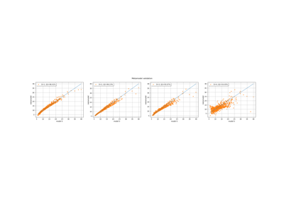
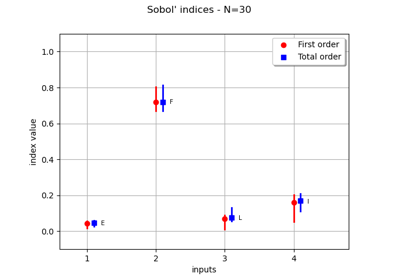
.Examples using the class

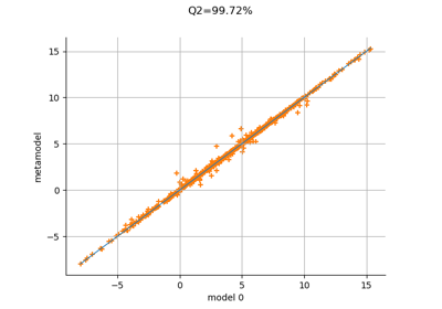

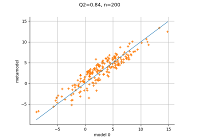
Create a full or sparse polynomial chaos expansion

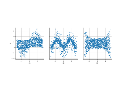
Create a polynomial chaos for the Ishigami function: a quick start guide to polynomial chaos
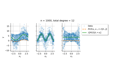
Conditional expectation of a polynomial chaos expansion
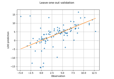
Compute leave-one-out error of a polynomial chaos expansion