ProcessSample¶

(Source code, png, hires.png, pdf)

class ProcessSample(*args)¶

Collection of fields.

Available constructors:

ProcessSample(mesh, K, d)

ProcessSample(mesh, coll)

ProcessSample(K, field)

Parameters:

meshMesh: The mesh shared by all the fields in the collection.
Kint: Number of fields in the collection.
dint: Dimension of the values of the field.
fieldField: One field.
collsequence of Sample: List of field values.

Notes

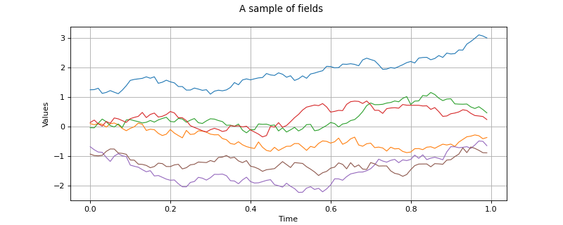
A ProcessSample stores a sample of fields. We note K the number of fields contained in the process sample and d the dimension of the values associated to each vertex of the common mesh $\cM \in \Rset^n$ .

These fields can be generated by a stochastic process.

In the first usage, we fix the common mesh with mesh, the number of fields contained in the sample with K and the dimension of the values with d. The values of the fields are by default fixed to zero.
In the second usage, the collection of fields is filled with K copies of the given field field.

We note $\vect{x}_i^k \in \Rset^d$ the value of the field k at the vertex i. We note N the number of vertices of $\cM$ , with $0 \leq i \leq N-1$ and $1 \leq k \leq K$ .

Examples

Create a bi dimensional mesh as a box:

>>> import openturns as ot
>>> myIndices = [10, 5]
>>> myMesher = ot.IntervalMesher(myIndices)
>>> lowerBound = [0.0, 0.0]
>>> upperBound = [2.0, 1.0]
>>> myInterval = ot.Interval(lowerBound, upperBound)
>>> myMesh = myMesher.build(myInterval)

Create a second order normal porcess of dimension 3:

>>> amplitude = [5]
>>> scale = [3, 3]
>>> model = ot.ExponentialModel(scale, amplitude)
>>> myProcess = ot.GaussianProcess(model, myMesh)

Generate a sample of different fields:

>>> n = 10
>>> mySampleFields = myProcess.getSample(n)

Duplicate the same field:

>>> myField = myProcess.getRealization()
>>> n = 10
>>> mySampleFields2 = ot.ProcessSample(n, myField)

Methods

`add`(*args)	Add a field to the collection.
`clear`()	Erase all field values.
`computeCentralMoment`(k)	Compute the central moment field of the collection of fields.
`computeEmpiricalCDF`(point[, tail])	Compute the empirical CDF field of the collection of fields.
`computeKurtosis`()	Compute the kurtosis field of the collection of fields.
`computeMean`()	Compute the mean field of the collection of fields.
`computeMedian`()	Compute the median field of the collection of fields.
`computeQuantilePerComponent`(*args)	Compute the quantile field of the collection of fields.
`computeRange`()	Compute the range field of the collection of fields.
`computeRawMoment`(k)	Compute the raw moment field of the collection of fields.
`computeSkewness`()	Compute the skewness field of the collection of fields.
`computeSpatialMean`()	Compute the spatial mean of the values of the fields.
`computeStandardDeviation`()	Compute the standard deviation field of the collection of fields.
`computeTemporalMean`()	Compute the temporal mean of the values of the fields.
`computeVariance`()	Compute the variance field of the collection of fields.
`draw`([interpolate])	Draw the whole field.
`drawCorrelation`()	Draw correlation between all marginals.
`drawMarginal`([index, interpolate])	Draw the selected field.
`drawMarginalCorrelation`(i, j)	Draw correlation between 2 marginals.
`erase`(*args)	Erase point(s) at or between index(es) (in-place).
`getClassName`()	Accessor to the object's name.
`getDimension`()	Get the dimension of the values of fields.
`getField`(i)	Field accessor.
`getId`()	Accessor to the object's id.
`getImplementation`()	Accessor to the underlying implementation.
`getMarginal`(*args)	Marginal sample accessor.
`getMax`()	Compute the max field of the collection of fields.
`getMesh`()	Get the mesh of the fields.
`getMin`()	Compute the min field of the collection of fields.
`getName`()	Accessor to the object's name.
`getSampleAtVertex`(index)	Extract sample at specific vertex of the mesh.
`getSize`()	Get the size of the collection of fields.
`getTimeGrid`()	Get the time grid of the fields.
`setField`(field, i)	Field accessor.
`setName`(name)	Accessor to the object's name.

computeCenteredMoment

__init__(*args)¶

add(*args)¶

Add a field to the collection.

Parameters:

fieldField: A new field to add. This field shares the same mesh and the same dimension as the other fields of the collection.

clear()¶: Erase all field values.

computeCentralMoment(k)¶

Compute the central moment field of the collection of fields.

Parameters:

kint: Order of the moment.

Returns:

momentField: This field has the same size and the same dimension as the fields of the collection. At each vertex of the mesh, we compute the component-wise central moment of order n.

computeEmpiricalCDF(point, tail=False)¶

Compute the empirical CDF field of the collection of fields.

Parameters:

pointsequence of float: The point at which all the marginal CDF are computed. Its dimension must match the process sample dimension.
tailbool (optional, default=False): Flag to if it is the CDF or the complementary CDF which is computed.

Returns:

cdfField: This field is scalar and has the same size as the process sample. At each vertex of the mesh, we compute the component-wise empirical CDF at the given point.

computeKurtosis()¶

Compute the kurtosis field of the collection of fields.

Returns:

kurtosisField: The squewness field has the same dimension d and the same mesh as the fields contained in the collection. At each vertex of the mesh, we compute the kurtosis of the values at this vertex of the K fields contained in the process sample.

computeMean()¶

Compute the mean field of the collection of fields.

Returns:

meanField: The mean field has the same dimension d and the same mesh as the fields contained in the collection. At each vertex of the mesh, we compute the mean of the values at this vertex of the K fields contained in the process sample:

$\forall i \in [0,N-1], \quad \dfrac{1}{K} \sum_{k=1}^K \vect{x}_i^k$

computeMedian()¶

Compute the median field of the collection of fields.

Returns:

medianField: This field has the same size and the same dimension as the fields of the collection. At each vertex of the mesh, we compute the component-wise empirical median. It is the same as computeQuantilePerComponent(0.5).

computeQuantilePerComponent(*args)¶

Compute the quantile field of the collection of fields.

Parameters:

pfloat, $0 \leq p \leq 1$ , or sequence of float: Order of the quantile.

Returns:

quantileField or ProcessSample: This field has the same size and the same dimension as the fields of the collection. At each vertex of the mesh, we compute the component-wise empirical quantile of order p.

computeRange()¶

Compute the range field of the collection of fields.

Returns:

rangeField: This field has the same size and the same dimension as the fields of the collection. At each vertex of the mesh, we compute the component-wise range, i.e. the difference between the largest and the lowest value in the field collection.

computeRawMoment(k)¶

Compute the raw moment field of the collection of fields.

Parameters:

kint: Order of the moment.

Returns:

momentField: This field has the same size and the same dimension as the fields of the collection. At each vertex of the mesh, we compute the component-wise raw moment of order n.

computeSkewness()¶

Compute the skewness field of the collection of fields.

Returns:

skewnessField: The squewness field has the same dimension d and the same mesh as the fields contained in the collection. At each vertex of the mesh, we compute the skewness of the values at this vertex of the K fields contained in the process sample.

computeSpatialMean()¶

Compute the spatial mean of the values of the fields.

Returns:

spatialMeanSample: Its size is the number K of fields in the collection. Its dimension is d. The k numerical point is the spatial mean of the field k:

$\forall k \in [1,K], \quad \dfrac{1}{N}\sum_{i=0}^{N-1} \vect{x}_i^k$

computeStandardDeviation()¶

Compute the standard deviation field of the collection of fields.

Returns:

stddevField: The standard deviation field has the same dimension d and the same mesh as the fields contained in the collection. At each vertex of the mesh, we compute the standard deviation of the values at this vertex of the K fields contained in the process sample:

$\forall i \in [0,N-1], \quad \sqrt{\dfrac{1}{K-1} \sum_{k=1}^K (\vect{x}_i^k - \hat{\mu}_i)^2}$

computeTemporalMean()¶

Compute the temporal mean of the values of the fields.

Returns:

spatialMeanSample: Its size is the number K of fields in the collection. Its dimension is d. The k numerical point is the temporal mean of the field k:

$\forall k \in [1,K], \quad \dfrac{1}{N}\sum_{i=0}^{N-1} \vect{x}_i^k$
This method can be used only when the mesh can be interpreted as a regular grid.

computeVariance()¶

Compute the variance field of the collection of fields.

Returns:

varianceField: The variance field has the same dimension d and the same mesh as the fields contained in the collection. At each vertex of the mesh, we compute the variance of the values at this vertex of the K fields contained in the process sample.

draw(interpolate=True)¶

Draw the whole field.

Parameters:

interpolatebool (optional, default=True): Whether to draw interpolated values.

Returns:

graphGridLayout: The graph of the whole field using the interpolate method.

drawCorrelation()¶

Draw correlation between all marginals.

This is only available on a 1-d mesh.

Returns:

graphGridLayout: The graph of the correlation between all marginals.

drawMarginal(index=0, interpolate=True)¶

Draw the selected field.

Parameters:

indiceint: Index of the field that is drawn in the graph.
interpolatebool (optional, default=True): Whether to draw interpolated values.

Returns:

graphGraph: The graph of the selected field using the interpolate method.

drawMarginalCorrelation(i, j)¶

Draw correlation between 2 marginals.

This is only available on a 1-d mesh.

Parameters:

i, jint, $i, j < d$: Marginal indices.

Returns:

graphGraph: The graph of the correlation between 2 marginals.

erase(*args)¶

Erase point(s) at or between index(es) (in-place).

Parameters:

fint, $0 \leq f < m$: The index of the first point to erase.
lint, $f < l \leq m$ , optional: The index after the last point to erase. Default uses l = f + 1 and only removes sample[f].

getClassName()¶

Accessor to the object’s name.

Returns:

class_namestr: The object class name (object.__class__.__name__).

getDimension()¶

Get the dimension of the values of fields.

Returns:

dint: Dimension of the values of the fields.

getField(i)¶

Field accessor.

Parameters:

iint: Field index

Returns:

fieldField: i-th field in the sample.

getId()¶

Accessor to the object’s id.

Returns:

idint: Internal unique identifier.

getImplementation()¶

Accessor to the underlying implementation.

Returns:

implImplementation: A copy of the underlying implementation object.

getMarginal(*args)¶

Marginal sample accessor.

Parameters:

indiceint or sequence of int: Index of the marginals.

Returns:

sampleProcessSample: The marginal sample.

getMax()¶

Compute the max field of the collection of fields.

Returns:

maxField: This field has the same size and the same dimension as the fields of the collection. At each vertex of the mesh, we compute the component-wise maximum.

getMesh()¶

Get the mesh of the fields.

Returns:

meshMesh: The mesh shared by all the fields of the collection.

getMin()¶

Compute the min field of the collection of fields.

Returns:

minField: This field has the same size and the same dimension as the fields of the collection. At each vertex of the mesh, we compute the component-wise minimum.

getName()¶

Accessor to the object’s name.

Returns:

namestr: The name of the object.

getSampleAtVertex(index)¶

Extract sample at specific vertex of the mesh.

Parameters:

indexint, $index < N$: Node index in the mesh.

Returns:

sample_at_iSample: The sample of all values of the trajectories at the desired node.

getSize()¶

Get the size of the collection of fields.

Returns:

Kint: Number of fields in the collection.

getTimeGrid()¶

Get the time grid of the fields.

Returns:

meshRegularGrid: The time grid shared by all the fields of the collection. Can be used only if the mesh can be interpreted as a regular time grid.

setField(field, i)¶

Field accessor.

Parameters: