Metamodel a FMU time-dependent output

We are interested in the evolution of an epidemic through a population (for instance, Covid!). We have an epidemiologic model describing the epidemic dynamics. More precisely, we focus on the evolution of the number of people infected by the disease.

---

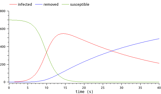
See the epidemiological model here.

---

To decrease the model simulation costs, let’s create a metamodel.

Metamodeling a model which output depends on time is a difficult problem. We will combine two methods: Karhunen-Loeve dimension reduction should precede the Kriging metamodeling.

We will proceed the following way:

• simulate the FMU n times on a design of experiment,

• concentrate the information of the time-dependent output via Karhunen-Loeve,

• metamodel the Karhunen-Loeve coefficients.

The composition of the coefficients metamodel with the inverse Karhunen-Loeve will make the global metamodel.

Create the metamodel

We load the FMU as a FMUPointToFieldFunction (see the tutorial). We concentrate on the first time unit of the epidemiological model output. The single uncertain input of the model is the ìnfection_rate.

import otfmi.example.utility
import openturns as ot
import openturns.viewer as viewer

path_fmu = otfmi.example.utility.get_path_fmu("epid")
mesh = ot.RegularGrid(0.0, 0.05, 20)
meshSample = mesh.getVertices()

function = otfmi.FMUPointToFieldFunction(
    mesh,
    path_fmu,
    inputs_fmu=["infection_rate"],
    outputs_fmu=["infected"],
    start_time=0.0,
    final_time=1.0,
)

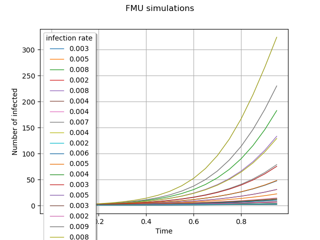
We create a Monte-Carlo design of experiment, on which we simulate the FMU. The simulation inputs and outputs will be used to train the metamodel.

inputLaw = ot.Uniform(0.001, 0.01)
inputSample = inputLaw.getSample(30)
outputFMUSample = function(inputSample)

graph = outputFMUSample.draw().getGraph(0, 0)
graph.setTitle("FMU simulations")
graph.setXTitle("Time")
graph.setYTitle("Number of infected")
graph.setLegends(["{:.3f}".format(line[0]) for line in inputSample])
view = viewer.View(graph, legend_kw={"title": "infection rate", "loc": "upper left"})
view.ShowAll()

We define a function to visualize the upcoming Karhunen-Loevem modes.

def drawKL(scaledKL, KLev, mesh, title="Scaled KL modes"):
    graph_modes = scaledKL.drawMarginal()
    graph_modes.setTitle(title + " scaled KL modes")
    graph_modes.setXTitle("$x$")
    graph_modes.setYTitle(r"$\sqrt{\lambda_i}\phi_i$")
    data_ev = [[i, KLev[i]] for i in range(scaledKL.getSize())]
    graph_ev = ot.Graph()
    graph_ev.add(ot.Curve(data_ev))
    graph_ev.add(ot.Cloud(data_ev))
    graph_ev.setTitle(title + " KL eigenvalues")
    graph_ev.setXTitle("$k$")
    graph_ev.setYTitle(r"$\lambda_i$")
    graph_ev.setAxes(True)
    graph_ev.setGrid(True)
    graph_ev.setLogScale(2)
    bb = graph_ev.getBoundingBox()
    lower = bb.getLowerBound()
    lower[1] = 1.0e-7
    bb = ot.Interval(lower, bb.getUpperBound())
    graph_ev.setBoundingBox(bb)
    return graph_modes, graph_ev

We compute the Karhunen-Loeve decomposition of the model outputs. The underlying assumption is that these outputs are realizations of a stochastic process.

threshold = 0.0001
algoKL = ot.KarhunenLoeveSVDAlgorithm(outputFMUSample, threshold)
algoKL.run()
resultKL = algoKL.getResult()

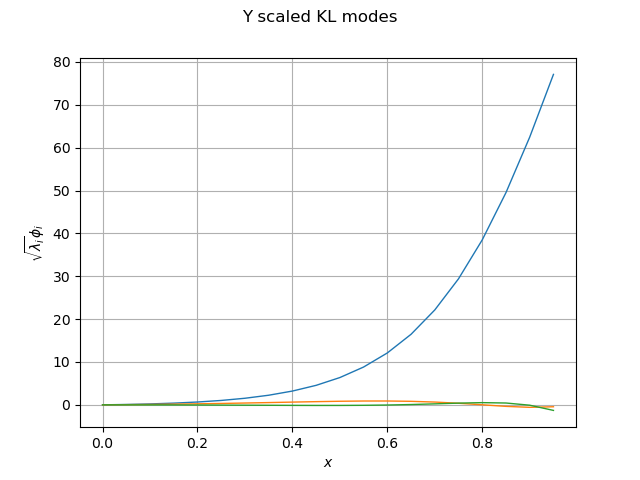
Let be curious and plot the Karhunen-Loeve modes:

phi_Y = resultKL.getScaledModesAsProcessSample()
lambda_Y = resultKL.getEigenvalues()
graph_modes_Y, graph_ev_Y = drawKL(phi_Y, lambda_Y, mesh, "Y")
view = viewer.View(graph_modes_Y)
view.ShowAll()

Now that Karhunen-Loeve algorithm is trained, we can project them in the smaller-dimension space:

projectionSample = resultKL.project(outputFMUSample)
n_mode = projectionSample.getDimension()
print("Karhunen-Loeve projection is dimension {}".format(n_mode))

Karhunen-Loeve projection is dimension 3

We keep on following our road map, by metamodeling the projection of the curves on the smaller-dimension space. We metamodel the Karhunen-Loeve coefficients using ordinary Kriging.

dim = inputSample.getDimension()  # only 1 input dimension
univb = ot.ConstantBasisFactory(dim).build()  # univariate basis
coll = [ot.AggregatedFunction([univb.build(i)] * n_mode) for i in range(univb.getSize())]
basis = ot.Basis(coll)  # multivariate basis
covarianceModel = ot.SquaredExponential(dim)
covarianceModel = ot.TensorizedCovarianceModel([covarianceModel] * n_mode)


algo = ot.KrigingAlgorithm(inputSample, projectionSample, covarianceModel, basis)
algo.run()
result = algo.getResult()
metamodel = result.getMetaModel()

We have created all pieces for a “PointToField” metamodel. Let put these pieces together:

def globalMetamodel(sample):
    emulatedCoefficients = metamodel(sample)
    restoreFunction = ot.KarhunenLoeveLifting(resultKL)
    emulatedProcessSample = restoreFunction(emulatedCoefficients)
    return emulatedProcessSample

Validate the metamodel

We create a new Monte-Carlo design of experiment. On this design of experiment, the FMU is simulated as well as the metamodel.

inputTestSample = inputLaw.getSample(10)
outputFMUTestSample = function(inputTestSample)
outputMetamodelTestSample = globalMetamodel(inputTestSample)

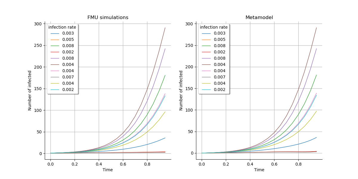
First, we have a visual check:

gridLayout = ot.GridLayout(1, 2)

graph1 = outputFMUTestSample.draw().getGraph(0, 0)
graph1.setTitle("FMU simulations")
graph2 = outputMetamodelTestSample.draw().getGraph(0, 0)
graph2.setTitle("Metamodel")

for graph in [graph1, graph2]:
    graph.setXTitle("Time")
    graph.setYTitle("Number of infected")
    graph.setLegends(["{:.3f}".format(line[0]) for line in inputSample])

gridLayout.setGraph(0, 0, graph1)
gridLayout.setGraph(0, 1, graph2)
view = viewer.View(
    gridLayout, legend_kw={"title": "infection rate", "loc": "upper left"}
)
view.ShowAll()

We validate the pertinence of Karhunen-Loeve decomposition:

validationKL = ot.KarhunenLoeveValidation(outputFMUTestSample, resultKL)
graph = validationKL.computeResidualMean().draw()
ot.Show(graph)

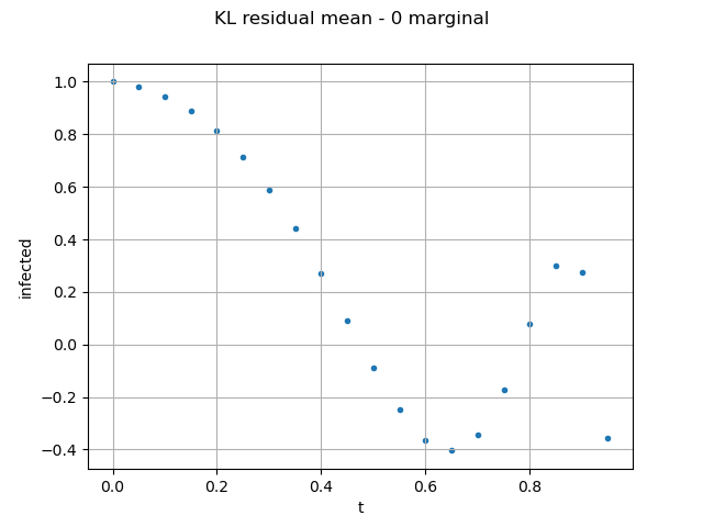
As the epidemiological model considers a population size of 700, the residual mean error on the field is acceptable.

We validate the Kriging (using the Karhunen-Loeve coefficients of the test sample):

projectFunction = ot.KarhunenLoeveProjection(resultKL)
coefficientSample = projectFunction(outputFMUTestSample)

validationKriging = ot.MetaModelValidation(
    inputTestSample, coefficientSample, metamodel
)
Q2 = validationKriging.computePredictivityFactor()[0]
print(Q2)

0.9999949331018687

The predictivity factor is very close to 1, which is satisfying. Further statistical tests exist in OpenTURNS to assert the quality of the obtained metamodel.

---

In this script, we have created and validated the globalMetamodel. This metamodel (computationnally faster than the FMU) can now be employed instead of the FMU to perform:

• sensitivity analysis,

• uncertainty propagation,

• estimate a failure probability,

etc.