FunctionalChaosResult
- class FunctionalChaosResult(*args)
Functional chaos result.
Returned by functional chaos algorithms, see
FunctionalChaosAlgorithm.- Parameters:
- sampleX2-d sequence of float
Input sample of
.
- sampleY2-d sequence of float
Output sample of
.
- distribution
Distribution Distribution of the random vector
- transformation
Function The function that maps the physical input
to the standardized input
.
- inverseTransformation
Function The function that maps the standardized input
to the physical input
.
- orthogonalBasis
OrthogonalBasis The multivariate orthogonal basis.
- indicessequence of int
The indices of the selected basis function within the orthogonal basis.
- alpha_k2-d sequence of float
The coefficients of the functional chaos expansion.
- Psi_ksequence of
Function The functions of the multivariate basis selected by the algorithm.
- residualssequence of float,
For each output component, the residual is the square root of the sum of squared differences between the model and the meta model, divided by the sample size.
- relativeErrorssequence of float,
The relative error is the empirical error divided by the sample variance of the output.
- isLeastSquaresbool
True if the expansion is computed using least squares.
- isModelSelectionbool
True if the expansion is computed using model selection.
Methods
Draw the error history.
Draw the basis selection history.
Accessor to the object's name.
Get the coefficients.
The coefficients values selection history accessor.
Get the composed metamodel.
getConditionalExpectation(conditioningIndices)Get the conditional expectation of the expansion given one vector input.
Get the input distribution.
The error history accessor.
Get the indices of the final basis.
The basis indices selection history accessor.
Accessor to the input sample.
Get the inverse isoprobabilistic transformation.
Accessor to the metamodel.
getName()Accessor to the object's name.
Get the orthogonal basis.
Accessor to the output sample.
Get the reduced basis.
Accessor to the relative errors.
Accessor to the residuals.
Get residuals sample.
Get the isoprobabilistic transformation.
hasName()Test if the object is named.
Get the model selection flag.
Get the least squares flag.
setErrorHistory(errorHistory)The error history accessor.
setInputSample(sampleX)Accessor to the input sample.
setInvolvesModelSelection(involvesModelSelection)Set the model selection flag.
setIsLeastSquares(isLeastSquares)Set the least squares flag.
setMetaModel(metaModel)Accessor to the metamodel.
setName(name)Accessor to the object's name.
setOutputSample(sampleY)Accessor to the output sample.
setRelativeErrors(relativeErrors)Accessor to the relative errors.
setResiduals(residuals)Accessor to the residuals.
setSelectionHistory(indicesHistory, ...)The basis coefficients and indices accessor.
Notes
Let
be the sample size. Let
be the dimension of the output of the physical model. For any
and any
, let
be the output of the physical model and let
be the output of the metamodel. For any
, let
be the sample output and let
be the output predicted by the metamodel. The marginal residual is:
for
, where
is the marginal sum of squares:
The marginal relative error is:
for
, where
is the unbiased sample variance of the
-th output.
This structure is created by the method run() of
FunctionalChaosAlgorithm, and obtained thanks to the getResult() method.- __init__(*args)
- drawErrorHistory()
Draw the error history.
This is only available with
LARS, and when the output dimension is 1.- Returns:
- graph
Graph The evolution of the error at each selection iteration
- graph
- drawSelectionHistory()
Draw the basis selection history.
This is only available with
LARS, and when the output dimension is 1.- Returns:
- graph
Graph The evolution of the basis coefficients at each selection iteration
- graph
- getClassName()
Accessor to the object’s name.
- Returns:
- class_namestr
The object class name (object.__class__.__name__).
- getCoefficients()
Get the coefficients.
- Returns:
- coefficients2-d sequence of float
Coefficients
.
- getCoefficientsHistory()
The coefficients values selection history accessor.
This is only available with
LARS, and when the output dimension is 1.- Returns:
- coefficientsHistory2-d sequence of float
The coefficients values selection history, for each iteration. Each inner list gives the coefficients values of the basis terms at i-th iteration.
- getComposedMetaModel()
Get the composed metamodel.
The composed metamodel is defined on the standard space
. It is defined by the equation:
for any
.
- Returns:
- composedMetamodel
Function The metamodel in the standard space
.
- composedMetamodel
- getConditionalExpectation(conditioningIndices)
Get the conditional expectation of the expansion given one vector input.
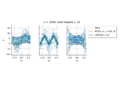
This method returns the functional chaos result corresponding to the conditional expectation of the output given an input vector. Indeed, the conditional expectation of a polynomial chaos expansion is, again, a polynomial chaos expansion. This is possible only if the marginals of the input distribution are independent. Otherwise, an exception is generated. An example is provided in Conditional expectation of a polynomial chaos expansion.
We consider the notations introduced in Functional Chaos Expansion. Let
be the input and let
be a set of marginal indices. Let
be the vector corresponding to the group of input variables where
is the number of input variables in the group. Let
be the polynomial chaos expansion of the physical model
. This function returns the functional chaos expansion of:
for any
.
Mathematical analysis
The mathematical derivation is better described in the standard space
than in the physical space
and this is why we consider the former. Assume that the basis functions
are defined by the tensor product:
for any
and any
where
is the set of orthonormal polynomials of degree
for the
-th input marginal. Assume that the PCE to order
is:
for any
. Assume that the input marginals
are independent. Let
be a group of variables with dimension
. Assume that
is the Cartesian product of vectors which have components in the group
and other components, i.e. assume that:
where
and
. Let
be the conditional expectation of the function
given
:
for any
. Let
be the set of multi-indices having zero components when the marginal multi-index is not in
:
This set of multi-indices defines the functions that depends on the variables in the group
and only them. For any
, let
be the orthogonal polynomial defined by :
Therefore :
for any
. Finally, the conditional expectation of the surrogate model is:
where
is the corresponding marginal mapping of the iso-probabilistic mapping
.
- Parameters:
- conditioningIndicessequence of int in [0, inputDimension - 1]
The indices
of the input random vector to condition.
- Returns:
- conditionalPCE
FunctionalChaosResult The functional chaos result of the conditional expectation. Its input dimension is
and its output dimension is
(i.e. the output dimension is unchanged).
- conditionalPCE
- getDistribution()
Get the input distribution.
- Returns:
- distribution
Distribution Distribution of the input random vector
.
- distribution
- getErrorHistory()
The error history accessor.
This is only available with
LARS, and when the output dimension is 1.- Returns:
- errorHistorysequence of float
The error history
- getIndices()
Get the indices of the final basis.
- Returns:
- indices
Indices Indices
of the elements of the multivariate basis used in the decomposition. Each integer in this list is the input argument of the
EnumerateFunction. If a model selection method such asLARSis used, these indices are not contiguous.
- indices
- getIndicesHistory()
The basis indices selection history accessor.
This is only available with
LARS, and when the output dimension is 1.- Returns:
- indicesHistory2-d sequence of int
The basis indices selection history, for each iteration. Each inner list gives the indices of the basis terms at i-th iteration.
- getInverseTransformation()
Get the inverse isoprobabilistic transformation.
- Returns:
- invTransf
Function such that
.
- invTransf
- getName()
Accessor to the object’s name.
- Returns:
- namestr
The name of the object.
- getOrthogonalBasis()
Get the orthogonal basis.
- Returns:
- basis
OrthogonalBasis Factory of the orthogonal basis.
- basis
- getReducedBasis()
Get the reduced basis.
- Returns:
- basislist of
Function Collection of the functions
used in the decomposition.
- basislist of
- getRelativeErrors()
Accessor to the relative errors.
- Returns:
- relativeErrors
Point The relative errors defined as follows for each output of the model:
with
the vector of the
model’s values
and
the metamodel’s values.
- relativeErrors
- getResiduals()
Accessor to the residuals.
- Returns:
- residuals
Point The residual values defined as follows for each output of the model:
with
the
model’s values and
the metamodel’s values.
- residuals
- getSampleResiduals()
Get residuals sample.
- Returns:
- residualsSample
Sample The sample of residuals
for
and
.
- residualsSample
- getTransformation()
Get the isoprobabilistic transformation.
- Returns:
- transformation
Function Transformation
such that
.
- transformation
- hasName()
Test if the object is named.
- Returns:
- hasNamebool
True if the name is not empty.
- involvesModelSelection()
Get the model selection flag.
A model selection method can be used to select the coefficients of the decomposition which enable to best predict the output. Model selection can lead to a sparse functional chaos expansion.
- Returns:
- involvesModelSelectionbool
True if the method involves a model selection method.
- isLeastSquares()
Get the least squares flag.
- Returns:
- isLeastSquaresbool
True if the coefficients were estimated from least squares.
- setErrorHistory(errorHistory)
The error history accessor.
- Parameters:
- errorHistorysequence of float
The error history
- setInputSample(sampleX)
Accessor to the input sample.
- Parameters:
- inputSample
Sample The input sample.
- inputSample
- setInvolvesModelSelection(involvesModelSelection)
Set the model selection flag.
A model selection method can be used to select the coefficients of the decomposition which enable to best predict the output. Model selection can lead to a sparse functional chaos expansion.
- Parameters:
- involvesModelSelectionbool
True if the method involves a model selection method.
- setIsLeastSquares(isLeastSquares)
Set the least squares flag.
- Parameters:
- isLeastSquaresbool
True if the coefficients were estimated from least squares.
- setName(name)
Accessor to the object’s name.
- Parameters:
- namestr
The name of the object.
- setOutputSample(sampleY)
Accessor to the output sample.
- Parameters:
- outputSample
Sample The output sample.
- outputSample
- setRelativeErrors(relativeErrors)
Accessor to the relative errors.
- Parameters:
- relativeErrorssequence of float
The relative errors defined as follows for each output of the model:
with
the vector of the
model’s values
and
the metamodel’s values.
- setResiduals(residuals)
Accessor to the residuals.
- Parameters:
- residualssequence of float
The residual values defined as follows for each output of the model:
with
the
model’s values and
the metamodel’s values.
- setSelectionHistory(indicesHistory, coefficientsHistory)
The basis coefficients and indices accessor.
- Parameters:
- indicesHistory2-d sequence of int
The basis indices selection history
- coefficientsHistory2-d sequence of float
The coefficients values selection history Must be of same size as indicesHistory.
Examples using the class

Create a full or sparse polynomial chaos expansion
Create a polynomial chaos metamodel by integration on the cantilever beam
Create a polynomial chaos metamodel from a data set
Create a polynomial chaos for the Ishigami function: a quick start guide to polynomial chaos
Conditional expectation of a polynomial chaos expansion
Example of sensitivity analyses on the wing weight model
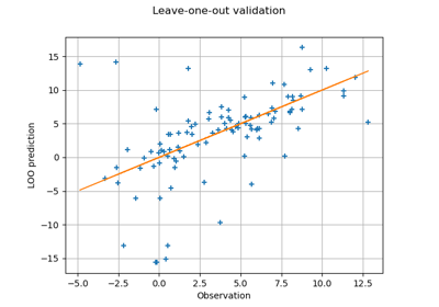
Compute leave-one-out error of a polynomial chaos expansion
 OpenTURNS


