SquareMatrix
- class SquareMatrix(*args)
Real square matrix.
- Parameters:
- sizeint,
 , optional
 Matrix size. Default is 1.
- valuessequence of float with size
 , optional
 Values. OpenTURNS uses column-major ordering (like Fortran) for reshaping the flat list of values. Default creates a zero matrix.
- sizeint,
Methods
clean(threshold)Set elements smaller than a threshold to zero.
Compute the determinant.
Compute the determinant in place.
Compute the eigenvalues decomposition (EVD).
Compute the eigenvalues decomposition (EVD) in place.
Compute eigenvalues.
Compute eigenvalues in place.
computeGram([transpose])Compute the associated Gram matrix.
computeHadamardProduct(other)Compute the Hadamard product matrix.
Compute the largest eigenvalue module.
Compute the logarithm of the absolute value of the determinant.
Compute the determinant in place.
computeQR([fullQR])Compute the QR factorization.
computeQRInPlace([fullQR])Compute the QR factorization in place.
computeSVD([fullSVD])Compute the singular values decomposition (SVD).
computeSVDInPlace([fullSVD])Compute the singular values decomposition (SVD).
Compute the singular values.
Compute the singular values in place.
Compute the sum of the matrix elements.
Compute the trace of the matrix.
Frobenius norm accessor.
Accessor to the object's name.
getDiagonal([k])Get the k-th diagonal of the matrix.
getDiagonalAsPoint([k])Get the k-th diagonal of the matrix.
Accessor to the dimension (the number of rows).
getId()Accessor to the object's id.
Accessor to the underlying implementation.
getName()Accessor to the object's name.
Accessor to the number of columns.
Accessor to the number of rows.
inverse()Compute the inverse of the matrix.
Test whether the matrix is diagonal or not.
isEmpty()Tell if the matrix is empty.
reshape(newRowDim, newColDim)Reshape the matrix.
reshapeInPlace(newRowDim, newColDim)Reshape the matrix, in place.
setDiagonal(*args)Set the k-th diagonal of the matrix.
setName(name)Accessor to the object's name.
solveLinearSystem(*args)Solve a square linear system whose the present matrix is the operator.
solveLinearSystemInPlace(*args)Solve a rectangular linear system whose the present matrix is the operator.
Square the Matrix, ie each element of the matrix is squared.
Transpose the matrix.
Examples
Create a matrix
>>> import openturns as ot
>>> M = ot.SquareMatrix(2, range(2 * 2))
>>> print(M)
[[ 0 2 ]
 [ 1 3 ]]
Get or set terms
>>> print(M[0, 0])
0.0
>>> M[0, 0] = 1.0
>>> print(M[0, 0])
1.0
>>> print(M[:, 0])
[[ 1 ]
 [ 1 ]]
Create a matrix from a square Numpy 2d-array (or matrix, or 2d-list)…
>>> import numpy as np
>>> np_2d_array = np.array([[1.0, 2.0], [3.0, 4.0]])
>>> ot_matrix = ot.SquareMatrix(np_2d_array)
and back
>>> np_matrix = np.matrix(ot_matrix)
Basic linear algebra operations (provided the dimensions are compatible)
>>> A = ot.Matrix([[1.0, 2.0], [3.0, 4.0], [5.0, 6.0]])
>>> B = ot.SquareMatrix(np.eye(2))
>>> C = ot.Matrix(3, 2, [1.0] * 3 * 2)
>>> print(A * B - C)
[[ 0 1 ]
 [ 2 3 ]
 [ 4 5 ]]
>>> A = ot.SquareMatrix([[1.0, 2.0], [3.0, 4.0]])
>>> print(A ** 2)
[[  7 10 ]
 [ 15 22 ]]
- __init__(*args)
- clean(threshold)
Set elements smaller than a threshold to zero.
- Parameters:
- thresholdfloat
Threshold for zeroing elements.
- Returns:
- cleaned_matrix
Matrix Input matrix with elements smaller than the threshold set to zero.
- cleaned_matrix
- computeDeterminant()
Compute the determinant.
- Returns:
- determinantfloat
The square matrix determinant.
Examples
>>> import openturns as ot
>>> A = ot.SquareMatrix([[1.0, 2.0], [3.0, 4.0]])
>>> A.computeDeterminant()
-2.0
- computeDeterminantInPlace()
Compute the determinant in place.
Similar to
computeDeterminant()but modifies the matrix in place to avoid copy.
- computeEV()
Compute the eigenvalues decomposition (EVD).
The eigenvalues decomposition of a square matrix
 with
size
with
size  reads:
where
 is an
is an  diagonal matrix and
 is an orthogonal matrix.
- Returns:
- eigen_values
ComplexCollection The vector of eigenvalues with size
that form the diagonal of
the matrix of the EVD.- Phi
SquareComplexMatrix The left matrix of the EVD.
- eigen_values
Notes
This uses LAPACK’S DGEEV.
Examples
>>> import openturns as ot
>>> import numpy as np
>>> M = ot.SquareMatrix([[1.0, 2.0], [3.0, 4.0]])
>>> eigen_values, Phi = M.computeEV()
>>> Lambda = ot.SquareComplexMatrix(M.getDimension())
>>> for i in range(eigen_values.getSize()):
...     Lambda[i, i] = eigen_values[i]
>>> # from scipy.linalg import inv # SquareComplexMatrix does not implement solveLinearSystem
>>> # Phi, Lambda = np.matrix(Phi), np.matrix(Lambda)
>>> # np.testing.assert_array_almost_equal(Phi * Lambda * inv(Phi), M)
- computeEVInPlace()
Compute the eigenvalues decomposition (EVD) in place.
Similar to
computeEVInPlace()but the matrix is modified in place to avoid copy.
- computeEigenValues()
Compute eigenvalues.
- Returns:
- eigenvalues
ComplexCollection Eigenvalues.
- eigenvalues
See also
Examples
>>> import openturns as ot
>>> M = ot.SquareMatrix([[1.0, 2.0], [3.0, 4.0]])
>>> M.computeEigenValues()
[(-0.372281,0),(5.37228,0)]
- computeEigenValuesInPlace()
Compute eigenvalues in place.
Similar to
computeEigenValues()but the matrix is modified in place to avoid copy.
- computeGram(transpose=True)
Compute the associated Gram matrix.
- Parameters:
- transposedbool
Tells if matrix is to be transposed or not. Default value is True
- Returns:
- MMT
Matrix The Gram matrix.
- MMT
Notes
When transposed is True, compute
 .
Otherwise, compute
.
Otherwise, compute  .
.Examples
>>> import openturns as ot
>>> M = ot.Matrix([[1.0, 2.0], [3.0, 4.0], [5.0, 6.0]])
>>> MtM = M.computeGram()
>>> print(MtM)
[[ 35 44 ]
 [ 44 56 ]]
>>> MMt = M.computeGram(False)
>>> print(MMt)
[[  5 11 17 ]
 [ 11 25 39 ]
 [ 17 39 61 ]]
- computeHadamardProduct(other)
Compute the Hadamard product matrix.
Notes
The matrix
 resulting from the Hadamard product (
also known as the elementwise product) of the matrices
resulting from the Hadamard product (
also known as the elementwise product) of the matrices
 and
and  is:
is:
for any
 and
and  .
.Examples
>>> import openturns as ot
>>> A = ot.Matrix([[1.0, 2.0], [3.0, 4.0]])
>>> B = ot.Matrix([[1.0, 2.0], [3.0, 4.0]])
>>> C = A.computeHadamardProduct(B)
>>> print(C)
[[  1  4 ]
 [  9 16 ]]
>>> print(B.computeHadamardProduct(A))
[[  1  4 ]
 [  9 16 ]]
- computeLargestEigenValueModule(*args)
Compute the largest eigenvalue module.
- Parameters:
- maximumIterationsint, optional
The maximum number of power iterations to perform to get the approximation. Default is given by the ‘Matrix-LargestEigenValueIterations’ key in the
ResourceMap.- epsilonfloat, optional
The target relative error. Default is given by the ‘Matrix-LargestEigenValueRelativeError’ key in the
ResourceMap.
- Returns:
- largestEigenvalueModulefloat
The largest eigenvalue module.
See also
Examples
>>> import openturns as ot
>>> M = ot.SquareMatrix([[1.0, 2.0], [3.0, 4.0]])
>>> M.computeLargestEigenValueModule()
5.3722...
- computeLogAbsoluteDeterminant()
Compute the logarithm of the absolute value of the determinant.
- Returns:
- determinantfloat
The logarithm of the absolute value of the square matrix determinant.
- signfloat
The sign of the determinant.
Examples
>>> import openturns as ot
>>> A = ot.SquareMatrix([[1.0, 2.0], [3.0, 4.0]])
>>> A.computeLogAbsoluteDeterminant()
[0.693147..., -1.0]
- computeLogAbsoluteDeterminantInPlace()
Compute the determinant in place.
Similar to
computeLogAbsoluteDeterminant()but modifies the matrix in place to avoid copy.
- computeQR(fullQR=False)
Compute the QR factorization.
By default, it is the economic decomposition which is computed. The economic QR factorization of a rectangular matrix
with
 (more rows than columns) is defined as follows:
where
 is an
is an  upper triangular matrix,
 is
is  ,
,  is
is
 , and and
both have orthogonal columns.
, and and
both have orthogonal columns.- Parameters:
- full_qrbool, optional
A flag telling whether Q, R or Q1, R1 are returned. Default is False and returns Q1, R1.
- Returns:
- Q1
Matrix The orthogonal matrix of the economic QR factorization.
- R1
TriangularMatrix The right (upper) triangular matrix of the economic QR factorization.
- Q
Matrix The orthogonal matrix of the full QR factorization.
- R
TriangularMatrix The right (upper) triangular matrix of the full QR factorization.
- Q1
Notes
The economic QR factorization is often used for solving overdetermined linear systems (where the operator
has ) in the
least-square sense because it implies solving a (simple) triangular system:
This uses LAPACK’s DGEQRF and DORGQR.
Examples
>>> import openturns as ot
>>> import numpy as np
>>> M = ot.Matrix([[1.0, 2.0], [3.0, 4.0], [5.0, 6.0]])
>>> Q1, R1 = M.computeQR()
>>> np.testing.assert_array_almost_equal(Q1 * R1, M)
- computeQRInPlace(fullQR=False)
Compute the QR factorization in place.
Similar to
computeQR()
- computeSVD(fullSVD=False)
Compute the singular values decomposition (SVD).
The singular values decomposition of a rectangular matrix
with
size  reads:
where
 is an
is an  orthogonal matrix,
 is an diagonal matrix and
 is an orthogonal matrix.
- Parameters:
- fullSVDbool, optional
Whether the null parts of the orthogonal factors are explicitly stored or not. Default is False and computes a reduced SVD.
- Returns:
- singular_values
Point The vector of singular values with size
 that
form the diagonal of the matrix
of the SVD.
that
form the diagonal of the matrix
of the SVD.- U
SquareMatrix The left orthogonal matrix of the SVD.
- VT
SquareMatrix The transposed right orthogonal matrix of the SVD.
- singular_values
Notes
This uses LAPACK’s DGESDD.
Examples
>>> import openturns as ot
>>> import numpy as np
>>> M = ot.Matrix([[1.0, 2.0], [3.0, 4.0], [5.0, 6.0]])
>>> singular_values, U, VT = M.computeSVD(True)
>>> Sigma = ot.Matrix(M.getNbRows(), M.getNbColumns())
>>> for i in range(singular_values.getSize()):
...     Sigma[i, i] = singular_values[i]
>>> np.testing.assert_array_almost_equal(U * Sigma * VT, M)
- computeSVDInPlace(fullSVD=False)
Compute the singular values decomposition (SVD).
Unlike computeSVD, this modifies the matrix in place and avoids a copy.
- computeSingularValues()
Compute the singular values.
- Parameters:
- fullSVDbool, optional
Whether the null parts of the orthogonal factors are explicitly stored or not. Default is False and computes a reduced SVD.
- Returns:
- singular_values
Point The vector of singular values with size
that
form the diagonal of the matrix
of the SVD decomposition.
- singular_values
See also
Examples
>>> import openturns as ot
>>> M = ot.Matrix([[1.0, 2.0], [3.0, 4.0], [5.0, 6.0]])
>>> print(M.computeSingularValues())
[9.52552,0.514301]
- computeSingularValuesInPlace()
Compute the singular values in place.
Similar to
computeSingularValues()but the matrix is modified in place to avoid copy.
- computeSumElements()
Compute the sum of the matrix elements.
- Returns:
- suma float
The sum of the elements.
Notes
Compute the sum of elements of the matrix
:
Examples
>>> import openturns as ot
>>> M = ot.Matrix([[1.0, 2.0], [3.0, 4.0], [5.0, 6.0]])
>>> s = M.computeSumElements()
>>> print(s)
21.0
- computeTrace()
Compute the trace of the matrix.
- Returns:
- tracefloat
The trace of the matrix.
Examples
>>> import openturns as ot
>>> M = ot.SquareMatrix([[1.0, 2.0], [3.0, 4.0]])
>>> M.computeTrace()
5.0
- frobeniusNorm()
Frobenius norm accessor.
- Returns:
- normfloat
The Frobenius norm
 .
.
- getClassName()
Accessor to the object’s name.
- Returns:
- class_namestr
The object class name (object.__class__.__name__).
- getDiagonal(k=0)
Get the k-th diagonal of the matrix.
- Parameters:
- kint
The k-th diagonal to extract Default value is 0
- Returns:
- D:
Matrix The k-th diagonal.
- D:
Examples
>>> import openturns as ot
>>> M = ot.Matrix([[1.0, 2.0, 3.0], [4.0, 5.0, 6.0], [7.0, 8.0, 9.0]])
>>> diag = M.getDiagonal()
>>> print(diag)
[[ 1 ]
 [ 5 ]
 [ 9 ]]
>>> print(M.getDiagonal(1))
[[ 2 ]
 [ 6 ]]
- getDiagonalAsPoint(k=0)
Get the k-th diagonal of the matrix.
- Parameters:
- kint
The k-th diagonal to extract Default value is 0
- Returns:
- pt
Point The k-th digonal.
- pt
Examples
>>> import openturns as ot
>>> M = ot.Matrix([[1.0, 2.0, 3.0], [4.0, 5.0, 6.0], [7.0, 8.0, 9.0]])
>>> pt = M.getDiagonalAsPoint()
>>> print(pt)
[1,5,9]
- getDimension()
Accessor to the dimension (the number of rows).
- Returns:
- dimensionint
- getId()
Accessor to the object’s id.
- Returns:
- idint
Internal unique identifier.
- getImplementation()
Accessor to the underlying implementation.
- Returns:
- implImplementation
A copy of the underlying implementation object.
- getName()
Accessor to the object’s name.
- Returns:
- namestr
The name of the object.
- getNbColumns()
Accessor to the number of columns.
- Returns:
- n_columnsint
- getNbRows()
Accessor to the number of rows.
- Returns:
- n_rowsint
- inverse()
Compute the inverse of the matrix.
- Returns:
- inverseMatrix
SquareMatrix The inverse of the matrix.
- inverseMatrix
Examples
>>> import openturns as ot
>>> M = ot.SquareMatrix([[1.0, 2.0, 3.0], [3.0, 2.0, 1.0], [2.0, 1.0, 3.0]])
>>> print(12.0 * M.inverse())
[[ -5  3  4 ]
 [  7  3 -8 ]
 [  1 -3  4 ]]
- isDiagonal()
Test whether the matrix is diagonal or not.
- Returns:
- testbool
Answer.
- isEmpty()
Tell if the matrix is empty.
- Returns:
- is_emptybool
True if the matrix contains no element.
Examples
>>> import openturns as ot
>>> M = ot.Matrix([[]])
>>> M.isEmpty()
True
- reshape(newRowDim, newColDim)
Reshape the matrix.
- Parameters:
- newRowDimint
The row dimension of the reshaped matrix.
- newColDimint
The column dimension of the reshaped matrix.
- Returns:
- MT
Matrix The reshaped matrix.
- MT
Notes
If the size of the reshaped matrix is smaller than the size of the matrix to be reshaped, only the
 first elements are kept (in
a column-major storage sense). If the size is greater, the new elements are set
to zero.
first elements are kept (in
a column-major storage sense). If the size is greater, the new elements are set
to zero.Examples
>>> import openturns as ot
>>> M = ot.Matrix([[1.0, 2.0], [3.0, 4.0], [5.0, 6.0]])
>>> print(M)
[[ 1 2 ]
 [ 3 4 ]
 [ 5 6 ]]
>>> print(M.reshape(1, 6))
1x6
[[ 1 3 5 2 4 6 ]]
>>> print(M.reshape(2, 2))
[[ 1 5 ]
 [ 3 2 ]]
>>> print(M.reshape(2, 6))
2x6
[[ 1 5 4 0 0 0 ]
 [ 3 2 6 0 0 0 ]]
- reshapeInPlace(newRowDim, newColDim)
Reshape the matrix, in place.
- Parameters:
- newRowDimint
The row dimension of the reshaped matrix.
- newColDimint
The column dimension of the reshaped matrix.
Notes
If the size of the reshaped matrix is smaller than the size of the matrix to be reshaped, only the
first elements are kept (in
a column-major storage sense). If the size is greater, the new elements are set
to zero. If the size is unchanged, no copy of data is done.Examples
>>> import openturns as ot
>>> M = ot.Matrix([[1.0, 2.0], [3.0, 4.0], [5.0, 6.0]])
>>> print(M)
[[ 1 2 ]
 [ 3 4 ]
 [ 5 6 ]]
>>> M.reshapeInPlace(1, 6)
>>> print(M)
1x6
[[ 1 3 5 2 4 6 ]]
>>> M.reshapeInPlace(2, 2)
>>> print(M)
[[ 1 5 ]
 [ 3 2 ]]
>>> M.reshapeInPlace(2, 6)
>>> print(M)
2x6
[[ 1 5 0 0 0 0 ]
 [ 3 2 0 0 0 0 ]]
- setDiagonal(*args)
Set the k-th diagonal of the matrix.
- Parameters:
Examples
>>> import openturns as ot
>>> M = ot.Matrix([[1.0, 2.0, 3.0], [4.0, 5.0, 6.0], [7.0, 8.0, 9.0]])
>>> M.setDiagonal([-1, 23, 9])
>>> print(M)
[[ -1  2  3 ]
 [  4 23  6 ]
 [  7  8  9 ]]
>>> M.setDiagonal(1.0)
>>> print(M)
[[ 1 2 3 ]
 [ 4 1 6 ]
 [ 7 8 1 ]]
>>> M.setDiagonal([2, 6, 9])
>>> print(M)
[[ 2 2 3 ]
 [ 4 6 6 ]
 [ 7 8 9 ]]
- setName(name)
Accessor to the object’s name.
- Parameters:
- namestr
The name of the object.
- solveLinearSystem(*args)
Solve a square linear system whose the present matrix is the operator.
- Parameters:
- rhssequence of float or
Matrixwith values or rows, respectively
 The right hand side member of the linear system.
- rhssequence of float or
- Returns:
Notes
This will handle both matrices and vectors. Note that you’d better type explicitly the matrix if it has some properties that could simplify the resolution (see
TriangularMatrix).This uses LAPACK’S DGESV for matrices and DGELSY for vectors.
Examples
>>> import openturns as ot
>>> import numpy as np
>>> M = ot.SquareMatrix([[1.0, 2.0], [3.0, 4.0]])
>>> b = [1.0] * 2
>>> x = M.solveLinearSystem(b)
>>> np.testing.assert_array_almost_equal(M * x, b)
- solveLinearSystemInPlace(*args)
Solve a rectangular linear system whose the present matrix is the operator.
Similar to
solveLinearSystem()except the matrix is modified in-place during the resolution avoiding the need to allocate an extra copy if the original copy is not re-used.
- squareElements()
Square the Matrix, ie each element of the matrix is squared.
Examples
>>> import openturns as ot
>>> M = ot.Matrix([[1.0, 2.0], [3.0, 4.0], [5.0, 6.0]])
>>> M.squareElements()
>>> print(M)
[[  1  4 ]
 [  9 16 ]
 [ 25 36 ]]
- transpose()
Transpose the matrix.
- Returns:
- MT
SquareMatrix The transposed matrix.
- MT
Examples
>>> import openturns as ot
>>> M = ot.SquareMatrix([[1.0, 2.0], [3.0, 4.0]])
>>> print(M)
[[ 1 2 ]
 [ 3 4 ]]
>>> print(M.transpose())
[[ 1 3 ]
 [ 2 4 ]]
Examples using the class


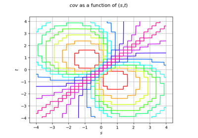
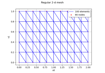
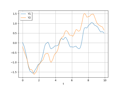
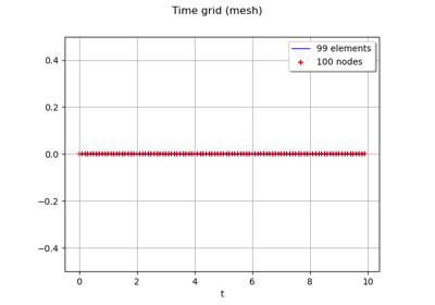
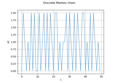
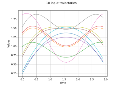
Sample trajectories from a Gaussian Process with correlated outputs


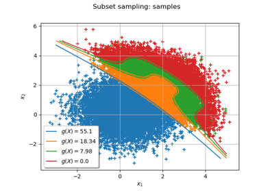
Use the post-analytical importance sampling algorithm

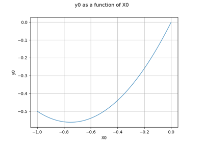
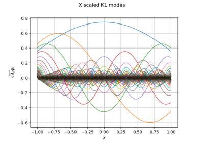
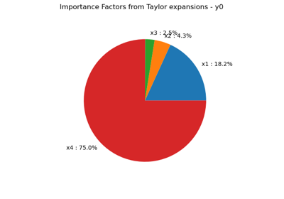
Estimate Sobol indices on a field to point function

Create mixed deterministic and probabilistic designs of experiments
Linear Regression with interval-censored observations