MetaModelAlgorithm
- class MetaModelAlgorithm(*args)
Base class for metamodel algorithms.
- Parameters:
- sampleX, sampleY2-d sequence of float
Input/output samples
- distribution
Distribution, optional Joint probability density function of the physical input vector.
Methods
BuildDistribution(inputSample)Recover the distribution, with metamodel performance in mind.
Accessor to the object's name.
Accessor to the joint probability density function of the physical input vector.
Accessor to the input sample.
getName()Accessor to the object's name.
Accessor to the output sample.
Return the weights of the input sample.
hasName()Test if the object is named.
run()Compute the response surfaces.
setDistribution(distribution)Accessor to the joint probability density function of the physical input vector.
setName(name)Accessor to the object's name.
See also
- __init__(*args)
- static BuildDistribution(inputSample)
Recover the distribution, with metamodel performance in mind.
For each marginal, find the best 1-d continuous parametric model else fallback to the use of a nonparametric one.
The selection is done as follow:
We start with a list of all parametric models (all factories)
For each model, we estimate its parameters if feasible.
We check then if model is valid, ie if its Kolmogorov score exceeds a threshold fixed in the MetaModelAlgorithm-PValueThreshold ResourceMap key. Default value is 5%
We sort all valid models and return the one with the optimal criterion.
For the last step, the criterion might be BIC, AIC or AICC. The specification of the criterion is done through the MetaModelAlgorithm-ModelSelectionCriterion ResourceMap key. Default value is fixed to BIC. Note that if there is no valid candidate, we estimate a non-parametric model (
KernelSmoothingorHistogram). The MetaModelAlgorithm-NonParametricModel ResourceMap key allows selecting the preferred one. Default value is HistogramOne each marginal is estimated, we use the Spearman independence test on each component pair to decide whether an independent copula. In case of non independence, we rely on a
NormalCopula.- Parameters:
- sample
Sample Input sample.
- sample
- Returns:
- distribution
Distribution Input distribution.
- distribution
- getClassName()
Accessor to the object’s name.
- Returns:
- class_namestr
The object class name (object.__class__.__name__).
- getDistribution()
Accessor to the joint probability density function of the physical input vector.
- Returns:
- distribution
Distribution Joint probability density function of the physical input vector.
- distribution
- getInputSample()
Accessor to the input sample.
- Returns:
- inputSample
Sample Input sample of a model evaluated apart.
- inputSample
- getName()
Accessor to the object’s name.
- Returns:
- namestr
The name of the object.
- getOutputSample()
Accessor to the output sample.
- Returns:
- outputSample
Sample Output sample of a model evaluated apart.
- outputSample
- getWeights()
Return the weights of the input sample.
- Returns:
- weightssequence of float
The weights of the points in the input sample.
- hasName()
Test if the object is named.
- Returns:
- hasNamebool
True if the name is not empty.
- run()
Compute the response surfaces.
Notes
It computes the response surfaces and creates a
MetaModelResultstructure containing all the results.
- setDistribution(distribution)
Accessor to the joint probability density function of the physical input vector.
- Parameters:
- distribution
Distribution Joint probability density function of the physical input vector.
- distribution
- setName(name)
Accessor to the object’s name.
- Parameters:
- namestr
The name of the object.
Examples using the class

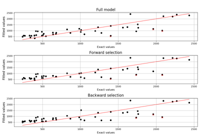


Create a full or sparse polynomial chaos expansion
Create a polynomial chaos metamodel by integration on the cantilever beam

Create a polynomial chaos metamodel from a data set
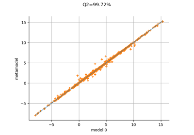
Create a polynomial chaos for the Ishigami function: a quick start guide to polynomial chaos
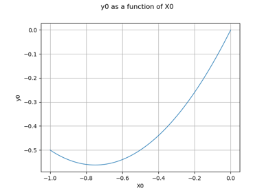
Conditional expectation of a polynomial chaos expansion

Gaussian Process Regression : cantilever beam model
Example of multi output Kriging on the fire satellite model
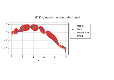
Kriging: choose a polynomial trend on the beam model

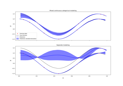
Kriging: metamodel with continuous and categorical variables
Example of sensitivity analyses on the wing weight model
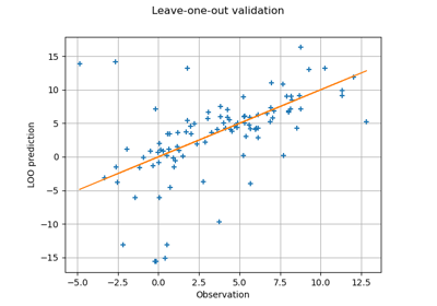
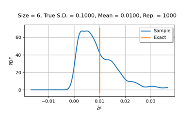
Compute leave-one-out error of a polynomial chaos expansion