Mesh¶

(Source code, png)

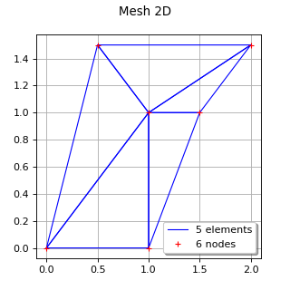
class Mesh(*args)¶

Mesh.

Available constructors:

Mesh(dim=1)

Mesh(vertices)

Mesh(vertices, simplices, checkValidity)

Parameters:

dimint, $dim \geq 0$: The dimension of the vertices. By default, it creates only one vertex of dimension $dim$ with components equal to 0.
vertices2-d sequence of float: Vertices’ coordinates in $\Rset^{dim}$ .
simplices2-d sequence of int: List of simplices defining the topology of the mesh. The simplex $[i_1, \dots, i_{dim+1}]$ connects the vertices of indices $(i_1, \dots, i_{dim+1})$ in $\Rset^{dim}$ . In dimension 1, a simplex is an interval $[i_1, i_2]$ ; in dimension 2, it is a triangle $[i_1, i_2, i_3]$ .
checkMeshValiditybool: Tells if we should check if mesh is valid i.e. if there is non-overlapping simplices, no unused vertex, no simplices with duplicate vertices and no coincident vertices. Default value is set to false in resource map key Mesh-CheckValidity

See also

RegularGrid

Examples

>>> import openturns as ot
>>> # Define the vertices of the mesh
>>> vertices = [[0.0, 0.0], [1.0, 0.0], [1.0, 1.0], [1.5, 1.0]]
>>> # Define the simplices of the mesh
>>> simplices = [[0, 1, 2], [1, 2, 3]]
>>> # Create the mesh of dimension 2
>>> mesh2d = ot.Mesh(vertices, simplices)

Methods

`ImportFromMSHFile`(fileName)	Import mesh from FreeFem 2-d mesh files.
`checkPointInSimplexWithCoordinates`(point, index)	Check if a point is inside a simplex and returns its barycentric coordinates.
`computeP1Gram`()	Compute the P1 Lagrange finite element gram matrix of the mesh.
`computeSimplicesVolume`()	Compute the volume of all simplices.
`computeWeights`()	Compute an approximation of an integral defined over the mesh.
`draw`()	Draw the mesh.
`draw1D`()	Draw the mesh of dimension 1.
`draw2D`()	Draw the mesh of dimension 2.
`draw3D`(*args)	Draw the bidimensional projection of the mesh.
`exportToVTKFile`(*args)	Export the mesh to a VTK file.
`fixOrientation`()	Make all the simplices positively oriented.
`getClassName`()	Accessor to the object's name.
`getDescription`()	Description accessor.
`getDimension`()	Dimension accessor.
`getId`()	Accessor to the object's id.
`getLowerBound`()	Lower bound accessor.
`getName`()	Accessor to the object's name.
`getShadowedId`()	Accessor to the object's shadowed id.
`getSimplex`(index)	Get the simplex of a given index.
`getSimplices`()	Get the simplices of the mesh.
`getSimplicesNumber`()	Get the number of simplices of the mesh.
`getUpperBound`()	Upper bound accessor.
`getVertex`(index)	Get the vertex of a given index.
`getVertices`()	Get the vertices of the mesh.
`getVerticesNumber`()	Get the number of vertices of the mesh.
`getVisibility`()	Accessor to the object's visibility state.
`getVolume`()	Get the volume of the mesh.
`hasName`()	Test if the object is named.
`hasVisibleName`()	Test if the object has a distinguishable name.
`isEmpty`()	Check whether the mesh is empty.
`isNumericallyEmpty`()	Check if the mesh is numerically empty.
`isRegular`()	Check if the mesh is regular (only for 1-d meshes).
`isValid`()	Check the mesh validity.
`setDescription`(description)	Description accessor.
`setName`(name)	Accessor to the object's name.
`setShadowedId`(id)	Accessor to the object's shadowed id.
`setSimplices`(simplices)	Set the simplices of the mesh.
`setVertex`(index, vertex)	Set a vertex of a given index.
`setVertices`(vertices)	Set the vertices of the mesh.
`setVisibility`(visible)	Accessor to the object's visibility state.
`streamToVTKFormat`(*args)	Give a VTK representation of the mesh.

__init__(*args)¶

static ImportFromMSHFile(fileName)¶

Import mesh from FreeFem 2-d mesh files.

Parameters:

MSHFilestr: A MSH ASCII file.

Returns:

meshMesh: Mesh defined in the file MSHFile.

checkPointInSimplexWithCoordinates(point, index)¶

Check if a point is inside a simplex and returns its barycentric coordinates.

Parameters:

pointsequence of float: Point of dimension $dim$ , the dimension of the vertices of the mesh.
indexint: Integer characterizes one simplex of the mesh.

Returns:

isInsidebool: Flag telling whether point is inside the simplex of index index.
coordinatesPoint: The barycentric coordinates of the given point wrt the vertices of the simplex.

Notes

The tolerance for the check on the barycentric coordinates can be tweaked using the key Mesh-CoordinateEpsilon.

Examples

>>> import openturns as ot
>>> vertices = [[0.0, 0.0], [1.0, 0.0], [1.0, 1.0]]
>>> simplex = [[0, 1, 2]]
>>> mesh2d = ot.Mesh(vertices, simplex)
>>> # Create a point A inside the simplex
>>> pointA = [0.6, 0.3]
>>> print(mesh2d.checkPointInSimplexWithCoordinates(pointA, 0))
[True, class=Point name=Unnamed dimension=3 values=[0.4,0.3,0.3]]
>>> # Create a point B outside the simplex
>>> pointB = [1.1, 0.6]
>>> print(mesh2d.checkPointInSimplexWithCoordinates(pointB, 0))
[False, class=Point name=Unnamed dimension=3 values=[-0.1,0.5,0.6]]

computeP1Gram()¶

Compute the P1 Lagrange finite element gram matrix of the mesh.

Returns:

gramCovarianceMatrix: P1 Lagrange finite element gram matrix of the mesh.

Notes

The P1 Lagrange finite element space associated to a mesh with vertices $(\vect{x}_i)_{i=1,\hdots,n}$ is the space of piecewise-linear functions generated by the functions $(\phi_i)_{i=1,\hdots,n}$ , where $\phi_i(\vect{x_i})=1$ , $\phi_i(\vect{x_j})=0$ for $j\neq i$ and the restriction of $\phi_i$ to any simplex is an affine function. The vertices that are not included into at least one simplex are not taken into account.

The gram matrix of the mesh is defined as the symmetric positive definite matrix $\mat{K}$ whose generic element $K_{i,j}$ is given by:

$\forall i,j=1,\hdots,n,\quad K_{i,j}=\int_{\cD}\phi_i(\vect{x})\phi_j(\vect{x})\di{\vect{x}}$

This method is used in several algorithms related to stochastic process representation such as the Karhunen-Loeve decomposition.

Examples

>>> import openturns as ot
>>> # Define the vertices of the mesh
>>> vertices = [[0.0, 0.0], [1.0, 0.0], [1.0, 1.0], [1.5, 1.0]]
>>> # Define the simplices of the mesh
>>> simplices = [[0, 1, 2], [1, 2, 3]]
>>> # Create the mesh of dimension 2
>>> mesh2d = ot.Mesh(vertices, simplices)
>>> print(mesh2d.computeP1Gram())
[[ 0.0833333 0.0416667 0.0416667 0         ]
 [ 0.0416667 0.125     0.0625    0.0208333 ]
 [ 0.0416667 0.0625    0.125     0.0208333 ]
 [ 0         0.0208333 0.0208333 0.0416667 ]]

computeSimplicesVolume()¶

Compute the volume of all simplices.

Returns:

volumePoint: Volume of all simplices.

Examples

>>> import openturns as ot
>>> vertices = [[0.0, 0.0], [1.0, 0.0], [1.0, 1.0]]
>>> simplex = [[0, 1, 2]]
>>> mesh2d = ot.Mesh(vertices, simplex)
>>> print(mesh2d.computeSimplicesVolume())
[0.5]

computeWeights()¶

Compute an approximation of an integral defined over the mesh.

Returns:

weightsPoint: Weights such that an integral of a function over the mesh is a weighted sum of its values at the vertices.

draw()¶

Draw the mesh.

Returns:

graphGraph: If the dimension of the mesh is 1, it draws the corresponding interval, using the draw1D() method; if the dimension is 2, it draws the triangular simplices, using the draw2D() method; if the dimension is 3, it projects the simplices on the plane of the two first components, using the draw3D() method with its default parameters, superposing the simplices.

draw1D()¶

Draw the mesh of dimension 1.

Returns:

graphGraph: Draws the line linking the vertices of the mesh when the mesh is of dimension 1.

Examples

>>> import openturns as ot
>>> from openturns.viewer import View
>>> vertices = [[0.5], [1.5], [2.1], [2.7]]
>>> simplices = [[0, 1], [1, 2], [2, 3]]
>>> mesh1d = ot.Mesh(vertices, simplices)
>>> # Create a graph
>>> aGraph = mesh1d.draw1D()
>>> # Draw the mesh
>>> View(aGraph).show()

draw2D()¶

Draw the mesh of dimension 2.

Returns:

graphGraph: Draws the edges of each simplex, when the mesh is of dimension 2.

Examples

>>> import openturns as ot
>>> from openturns.viewer import View
>>> vertices = [[0.0, 0.0], [1.0, 0.0], [1.0, 1.0], [1.5, 1.0]]
>>> simplices = [[0, 1, 2], [1, 2, 3]]
>>> mesh2d = ot.Mesh(vertices, simplices)
>>> # Create a graph
>>> aGraph = mesh2d.draw2D()
>>> # Draw the mesh
>>> View(aGraph).show()

draw3D(*args)¶

Draw the bidimensional projection of the mesh.

Available usages:

draw3D(drawEdge=True, thetaX=0.0, thetaY=0.0, thetaZ=0.0, shading=False, rho=1.0)

draw3D(drawEdge, rotation, shading, rho)

Parameters:

drawEdgebool: Tells if the edge of each simplex has to be drawn.
thetaXfloat: Gives the value of the rotation along the X axis in radian.
thetaYfloat: Gives the value of the rotation along the Y axis in radian.
thetaZfloat: Gives the value of the rotation along the Z axis in radian.
rotationSquareMatrix: Operates a rotation on the mesh before its projection of the plane of the two first components.
shadingbool: Enables to give a visual perception of depth and orientation.
rhofloat, $0 \leq \rho \leq 1$: Contraction factor of the simplices. If $\rho < 1$ , all the simplices are contracted and appear deconnected: some holes are created, which enables to see inside the mesh. If $\rho = 1$ , the simplices keep their initial size and appear connected. If $\rho = 0$ , each simplex is reduced to its gravity center.

Returns:

graphGraph: Draws the bidimensional projection of the mesh on the $(x,y)$ plane.

Examples

>>> import openturns as ot
>>> from openturns.viewer import View
>>> from math import cos, sin, pi
>>> vertices = [[0.0, 0.0, 0.0], [0.0, 0.0, 1.0], [0.0, 1.0, 0.0],
...             [0.0, 1.0, 1.0], [1.0, 0.0, 0.0], [1.0, 0.0, 1.0],
...             [1.0, 1.0, 0.0], [1.0, 1.0, 1.0]]
>>> simplices = [[0, 1, 2, 4], [3, 5, 6, 7],[1, 2, 3, 6],
...              [1, 2, 4, 6], [1, 3, 5, 6], [1, 4, 5, 6]]
>>> mesh3d = ot.Mesh(vertices, simplices)
>>> # Create a graph
>>> aGraph = mesh3d.draw3D()
>>> # Draw the mesh
>>> View(aGraph).show()
>>> rotation = ot.SquareMatrix(3)
>>> rotation[0, 0] = cos(pi / 3.0)
>>> rotation[0, 1] = sin(pi / 3.0)
>>> rotation[1, 0] = -sin(pi / 3.0)
>>> rotation[1, 1] = cos(pi / 3.0)
>>> rotation[2, 2] = 1.0
>>> # Create a graph
>>> aGraph = mesh3d.draw3D(True, rotation, True, 1.0)
>>> # Draw the mesh
>>> View(aGraph).show()

exportToVTKFile(*args)¶

Export the mesh to a VTK file.

Parameters:

myVTKFile.vtkstr: Name of the created file which contains the mesh and the associated random values that can be visualized with the open source software Paraview.

fixOrientation()¶

Make all the simplices positively oriented.

Examples

>>> import openturns as ot
>>> vertices = [[0.0, 0.0], [1.0, 0.0], [1.0, 1.0]]
>>> simplex = [[0, 2, 1]]
>>> mesh2d = ot.Mesh(vertices, simplex)
>>> print(mesh2d)
class=Mesh name=Unnamed dimension=2 vertices=class=Sample name=Unnamed implementation=class=SampleImplementation name=Unnamed size=3 dimension=2 data=[[0,0],[1,0],[1,1]] simplices=[[0,2,1]]
>>> mesh2d.fixOrientation()
>>> print(mesh2d)
class=Mesh name=Unnamed dimension=2 vertices=class=Sample name=Unnamed implementation=class=SampleImplementation name=Unnamed size=3 dimension=2 data=[[0,0],[1,0],[1,1]] simplices=[[2,0,1]]

getClassName()¶

Accessor to the object’s name.

Returns:

class_namestr: The object class name (object.__class__.__name__).

getDescription()¶

Description accessor.

Returns:

descriptionDescription: Description of the vertices.

Examples

>>> import openturns as ot
>>> mesh = ot.Mesh()
>>> vertices = ot.Sample([[0.0, 0.0], [1.0, 0.0], [1.0, 1.0]])
>>> vertices.setDescription(['X', 'Y'])
>>> mesh.setVertices(vertices)
>>> print(mesh.getDescription())
[X,Y]

getDimension()¶

Dimension accessor.

Returns:

dimensionint: Dimension of the vertices.

getId()¶

Accessor to the object’s id.

Returns:

idint: Internal unique identifier.

getLowerBound()¶

Lower bound accessor.

Returns:

lower_boundPoint: Min of the vertices.

getName()¶

Accessor to the object’s name.

Returns:

namestr: The name of the object.

getShadowedId()¶

Accessor to the object’s shadowed id.

Returns:

idint: Internal unique identifier.

getSimplex(index)¶

Get the simplex of a given index.

Parameters:

indexint: Index characterizing one simplex of the mesh.

Returns:

indicesIndices: Indices defining the simplex of index index. The simplex $[i_1, \dots, i_{n+1}]$ relies the vertices of index $(i_1, \dots, i_{n+1})$ in $\Rset^{dim}$ . In dimension 1, a simplex is an interval $[i_1, i_2]$ ; in dimension 2, it is a triangle $[i_1, i_2, i_3]$ .

Examples

>>> import openturns as ot
>>> vertices = [[0.0, 0.0], [1.0, 0.0], [1.0, 1.0], [1.5, 1.0]]
>>> simplices = [[0, 1, 2], [1, 2, 3]]
>>> mesh2d = ot.Mesh(vertices, simplices)
>>> print(mesh2d.getSimplex(0))
[0,1,2]
>>> print(mesh2d.getSimplex(1))
[1,2,3]

getSimplices()¶

Get the simplices of the mesh.

Returns:

indicesCollectioncollection of Indices: List of indices defining all the simplices. The simplex $[i_1, \dots, i_{n+1}]$ relies the vertices of index $(i_1, \dots, i_{n+1})$ in $\Rset^{dim}$ . In dimension 1, a simplex is an interval $[i_1, i_2]$ ; in dimension 2, it is a triangle $[i_1, i_2, i_3]$ .

Examples

>>> import openturns as ot
>>> vertices = [[0.0, 0.0], [1.0, 0.0], [1.0, 1.0], [1.5, 1.0]]
>>> simplices = [[0, 1, 2], [1, 2, 3]]
>>> mesh2d = ot.Mesh(vertices, simplices)
>>> print(mesh2d.getSimplices())
[[0,1,2],[1,2,3]]

getSimplicesNumber()¶

Get the number of simplices of the mesh.

Returns:

numberint: Number of simplices of the mesh.

getUpperBound()¶

Upper bound accessor.

Returns:

upper_boundPoint: Max of the vertices.

getVertex(index)¶

Get the vertex of a given index.

Parameters:

indexint: Index characterizing one vertex of the mesh.

Returns:

vertexPoint: Coordinates in $\Rset^{dim}$ of the vertex of index index, where $dim$ is the dimension of the vertices of the mesh.

Examples

>>> import openturns as ot
>>> vertices = [[0.0, 0.0], [1.0, 0.0], [1.0, 1.0]]
>>> simplices = [[0, 1, 2]]
>>> mesh2d = ot.Mesh(vertices, simplices)
>>> print(mesh2d.getVertex(1))
[1,0]
>>> print(mesh2d.getVertex(0))
[0,0]

getVertices()¶

Get the vertices of the mesh.

Returns:

verticesSample: Coordinates in $\Rset^{dim}$ of the vertices, where $dim$ is the dimension of the vertices of the mesh.

Examples

>>> import openturns as ot
>>> vertices = [[0.0, 0.0], [1.0, 0.0], [1.0, 1.0]]
>>> simplices = [[0, 1, 2]]
>>> mesh2d = ot.Mesh(vertices, simplices)
>>> print(mesh2d.getVertices())
0 : [ 0 0 ]
1 : [ 1 0 ]
2 : [ 1 1 ]

getVerticesNumber()¶

Get the number of vertices of the mesh.

Returns:

numberint: Number of vertices of the mesh.

getVisibility()¶

Accessor to the object’s visibility state.

Returns:

visiblebool: Visibility flag.

getVolume()¶

Get the volume of the mesh.

Returns:

volumefloat: Geometrical volume of the mesh which is the sum of its simplices’ volumes.

Examples

>>> import openturns as ot
>>> vertices = [[0.0, 0.0], [1.0, 0.0], [1.0, 1.0], [1.5, 1.0]]
>>> simplices = [[0, 1, 2], [1, 2, 3]]
>>> mesh2d = ot.Mesh(vertices, simplices)
>>> mesh2d.getVolume()
0.75

hasName()¶

Test if the object is named.

Returns:

hasNamebool: True if the name is not empty.

hasVisibleName()¶

Test if the object has a distinguishable name.

Returns:

hasVisibleNamebool: True if the name is not empty and not the default one.

isEmpty()¶

Check whether the mesh is empty.

Returns:

emptybool: Tells if the mesh is empty, ie if its volume is null.

isNumericallyEmpty()¶

Check if the mesh is numerically empty.

Returns:

isEmptybool: Flag telling whether the mesh is numerically empty, i.e. if its numerical volume is inferior or equal to $\epsilon$ (defined in the ResourceMap: $\epsilon$ = Domain-SmallVolume).

Examples

>>> import openturns as ot
>>> vertices = [[0.0, 0.0], [1.0, 0.0], [1.0, 1.0]]
>>> simplex = [[0, 1, 2]]
>>> mesh2d = ot.Mesh(vertices, simplex)
>>> print(mesh2d.isNumericallyEmpty())
False

isRegular()¶

Check if the mesh is regular (only for 1-d meshes).

Returns:

isRegularbool: Tells if the mesh is regular or not.

Examples

>>> import openturns as ot
>>> vertices = [[0.5], [1.5], [2.4], [3.5]]
>>> simplices = [[0, 1], [1, 2], [2, 3]]
>>> mesh1d = ot.Mesh(vertices, simplices)
>>> print(mesh1d.isRegular())
False
>>> vertices = [[0.5], [1.5], [2.5], [3.5]]
>>> mesh1d = ot.Mesh(vertices, simplices)
>>> print(mesh1d.isRegular())
True

isValid()¶

Check the mesh validity.

Returns:

validitybool: Tells if the mesh is valid i.e. if there is non-overlaping simplices, no unused vertex, no simplices with duplicate vertices and no coincident vertices.

setDescription(description)¶

Description accessor.

Parameters:

descriptionsequence of str: Description of the vertices.

Examples

>>> import openturns as ot
>>> mesh = ot.Mesh()
>>> vertices = ot.Sample([[0.0, 0.0], [1.0, 0.0], [1.0, 1.0]])
>>> mesh.setVertices(vertices)
>>> mesh.setDescription(['X', 'Y'])
>>> print(mesh.getDescription())
[X,Y]

setName(name)¶

Accessor to the object’s name.

Parameters:

namestr: The name of the object.

setShadowedId(id)¶

Accessor to the object’s shadowed id.

Parameters:

idint: Internal unique identifier.

setSimplices(simplices)¶

Set the simplices of the mesh.

Parameters:

indices2-d sequence of int: List of indices defining all the simplices. The simplex $[i_1, \dots, i_{n+1}]$ relies the vertices of index $(i_1, \dots, i_{n+1})$ in $\Rset^{dim}$ . In dimension 1, a simplex is an interval $[i_1, i_2]$ ; in dimension 2, it is a triangle $[i_1, i_2, i_3]$ .

Examples

>>> import openturns as ot
>>> mesh = ot.Mesh()
>>> simplices = [[0, 1, 2], [1, 2, 3]]
>>> mesh.setSimplices(simplices)

setVertex(index, vertex)¶

Set a vertex of a given index.

Parameters:

indexint: Index of the vertex to set.
vertexsequence of float: Cordinates in $\Rset^{dim}$ of the vertex of index index, where $dim$ is the dimension of the vertices of the mesh.

Examples

>>> import openturns as ot
>>> vertices = [[0.0, 0.0], [1.0, 0.0], [1.0, 1.0]]
>>> simplices = [[0, 1, 2]]
>>> mesh = ot.Mesh(vertices, simplices)
>>> vertex = [0.0, 0.5]
>>> mesh.setVertex(0, vertex)
>>> print(mesh.getVertices())
0 : [ 0   0.5 ]
1 : [ 1   0   ]
2 : [ 1   1   ]

setVertices(vertices)¶

Set the vertices of the mesh.

Parameters:

vertices2-d sequence of float: Cordinates in $\Rset^{dim}$ of the vertices, where $dim$ is the dimension of the vertices of the mesh.

Examples

>>> import openturns as ot
>>> mesh = ot.Mesh()
>>> vertices = [[0.0, 0.0], [1.0, 0.0], [1.0, 1.0]]
>>> mesh.setVertices(vertices)

setVisibility(visible)¶

Accessor to the object’s visibility state.

Parameters:

visiblebool: Visibility flag.

streamToVTKFormat(*args)¶

Give a VTK representation of the mesh.

Returns:

streamstr: VTK representation of the mesh.

Examples using the class¶

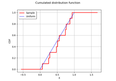
Kolmogorov-Smirnov : understand the p-value

Kolmogorov-Smirnov : get the statistics distribution

Estimate a multivariate ARMA process

Estimate a non stationary covariance function

Estimate a scalar ARMA process

Estimate a spectral density function

Estimate a stationary covariance function

Create a functional basis process

Add a trend to a process

Export a field to VTK

Aggregate processes

Create a gaussian process from a cov. model using HMatrix

Create a white noise process

Create a custom covariance model

Create a discrete Markov chain process

Manipulate a time series

Use the Box-Cox transformation

Create a stationary covariance model

Create a normal process

Create a random walk process

Create a spectral model

Draw a field

Create a process from random vectors and processes

Sample trajectories from a Gaussian Process with correlated outputs

Draw fields

Create and manipulate an ARMA process

Trend computation

Compare covariance models

Create a mesh

Over-fitting and model selection

Kriging : generate trajectories from a metamodel

Kriging : quick-start

Sequentially adding new points to a kriging

Kriging : choose a trend vector space

Kriging : draw covariance models

Validation of a Karhunen-Loeve decomposition

Viscous free fall: metamodel of a field function

Metamodel of a field function

Create a threshold event

Time variant system reliability problem

Create an event based on a process

Estimate a process-based event probability

Estimate Sobol indices on a field to point function

Value function

Vertex value function

Define a function with a field output: the viscous free fall example

Define a connection function with a field output

Logistic growth model

Generate flooding model observations

Generate observations of the Chaboche mechanical model

Bayesian calibration of a computer code

Customize your Metropolis-Hastings algorithm

Compute confidence intervals of a univariate noisy function

How to fill an area

A quick start guide to graphs

OpenTURNS

An Open source initiative for the Treatment of Uncertainties, Risks'N Statistics

Table of Contents

Previous topic

Next topic

This Page

Mesh¶

Examples using the class¶