View
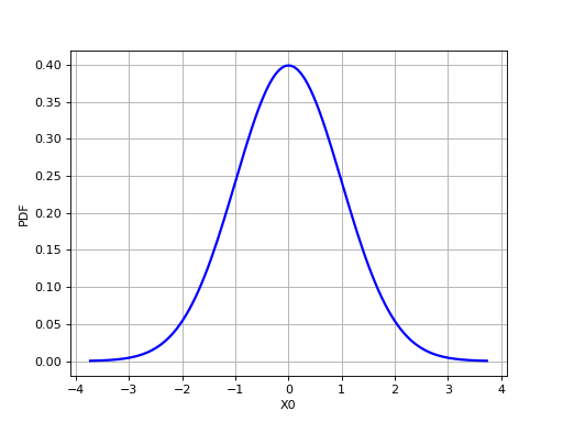
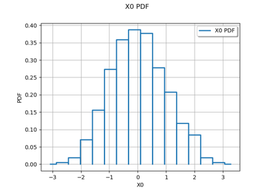
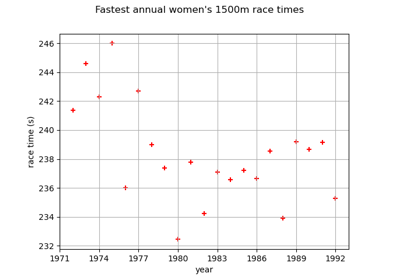
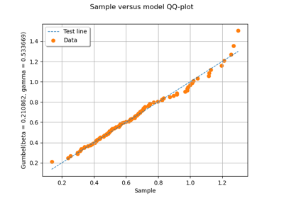
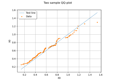
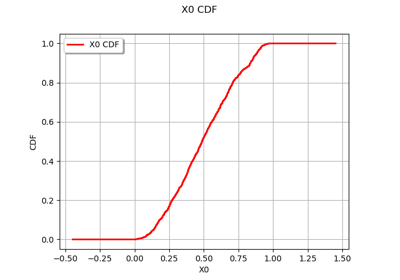
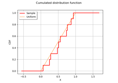
(Source code, png)
- class View(graph, pixelsize=None, figure=None, figure_kw=None, axes=[], plot_kw=None, axes_kw=None, bar_kw=None, pie_kw=None, polygon_kw=None, polygoncollection_kw=None, contour_kw=None, step_kw=None, clabel_kw=None, scatter_kw=None, text_kw=None, legend_kw=None, add_legend=True, square_axes=False, **kwargs)
Create the figure.
- Parameters:
- graph
Graph,DrawableorGridLayout An object to draw.
- pixelsize2-tuple of int
The requested size in pixels (width, height).
- figure
matplotlib.figure.Figure The figure to draw on.
- figure_kwdict, optional
Passed on to matplotlib.pyplot.figure kwargs
- axes
matplotlib.axes.Axes The axes to draw on.
- plot_kwdict, optional
Used when drawing Curve drawables Passed on as matplotlib.axes.Axes.plot kwargs
- axes_kwdict, optional
Passed on to matplotlib.figure.Figure.add_subplot kwargs
- bar_kwdict, optional
Used when drawing BarPlot drawables Passed on to matplotlib.pyplot.bar kwargs
- pie_kwdict, optional
Used when drawing Pie drawables Passed on to matplotlib.pyplot.pie kwargs
- polygon_kwdict, optional
Used when drawing Polygon drawables Passed on to matplotlib.patches.Polygon kwargs
- polygoncollection_kwdict, optional
Used when drawing PolygonArray drawables Passed on to matplotlib.collection.PolygonCollection kwargs
- contour_kwdict, optional
Used when drawing Contour drawables Passed on to matplotlib.pyplot.contour kwargs
- clabel_kwdict, optional
Used when drawing Contour drawables Passed on to matplotlib.pyplot.clabel kwargs
- scatter_kwdict, optional
Used when drawing Cloud drawables Passed on to matplotlib.pyplot.scatter kwargs
- step_kwdict, optional
Used when drawing Staircase drawables Passed on to matplotlib.pyplot.step kwargs
- text_kwdict, optional
Used when drawing Pairs, Text drawables Passed on to matplotlib.axes.Axes.text kwargs
- legend_kwdict, optional
Passed on to matplotlib.axes.Axes.legend kwargs
- add_legendbool, optional
Adds a legend if True. Default is True.
- square_axesbool, optional
Forces the axes to share the same scale if True. Default is False.
- graph
Examples
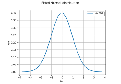
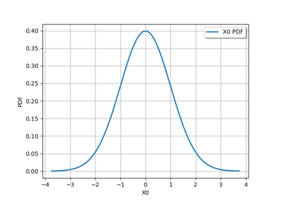
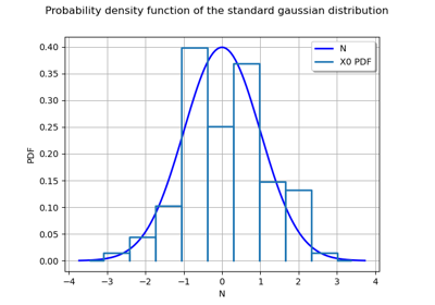
>>> import openturns as ot
>>> from openturns.viewer import View
>>> graph = ot.Normal().drawPDF()
>>> view = View(graph, plot_kw={'color':'blue'})
>>> view.save('graph.png', dpi=100)
>>> view.show()
Methods
ShowAll(**kwargs)Display all graphs.
close()Close the figure.
getAxes()Get the list of Axes objects.
Accessor to the underlying figure object.
save(fname, **kwargs)Save the graph as file.
show(**kwargs)Display the graph.
- __init__(graph, pixelsize=None, figure=None, figure_kw=None, axes=[], plot_kw=None, axes_kw=None, bar_kw=None, pie_kw=None, polygon_kw=None, polygoncollection_kw=None, contour_kw=None, step_kw=None, clabel_kw=None, scatter_kw=None, text_kw=None, legend_kw=None, add_legend=True, square_axes=False, **kwargs)
- static ShowAll(**kwargs)
Display all graphs.
Examples
>>> import openturns as ot
>>> import openturns.viewer as otv
>>> n = ot.Normal()
>>> graph = n.drawPDF()
>>> view = otv.View(graph)
>>> u = ot.Uniform()
>>> graph = u.drawPDF()
>>> view = otv.View(graph)
>>> otv.View.ShowAll()
- close()
Close the figure.
Examples
>>> import openturns as ot
>>> import openturns.viewer as otv
>>> n = ot.Normal()
>>> graph = n.drawPDF()
>>> view = otv.View(graph)
>>> view.close()
- getAxes()
Get the list of Axes objects.
See matplotlib.axes.Axes for further information.
Examples
>>> import openturns as ot
>>> import openturns.viewer as otv
>>> n = ot.Normal()
>>> graph = n.drawPDF()
>>> view = otv.View(graph)
>>> axes = view.getAxes()
>>> _ = axes[0].set_ylim(-0.1, 1.0);
- getFigure()
Accessor to the underlying figure object.
See matplotlib.figure.Figure for further information.
Examples
>>> import openturns as ot
>>> from openturns.viewer import View
>>> graph = ot.Normal().drawPDF()
>>> view = View(graph)
>>> fig = view.getFigure()
>>> _ = fig.suptitle("The suptitle");
- save(fname, **kwargs)
Save the graph as file.
- Parameters:
- fname: bool, optional
A string containing a path to a filename from which file format is deduced.
- kwargs:
See matplotlib.figure.Figure.savefig documentation for valid keyword arguments.
Examples
>>> import openturns as ot
>>> from openturns.viewer import View
>>> graph = ot.Normal().drawPDF()
>>> view = View(graph)
>>> view.save('graph.png', dpi=100)
- show(**kwargs)
Display the graph.
See matplotlib.figure.Figure.show
Examples
>>> import openturns as ot
>>> import openturns.viewer as otv
>>> n = ot.Normal()
>>> graph = n.drawPDF()
>>> view = otv.View(graph)
>>> view.show()
Examples using the class
Kolmogorov-Smirnov : get the statistics distribution
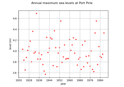
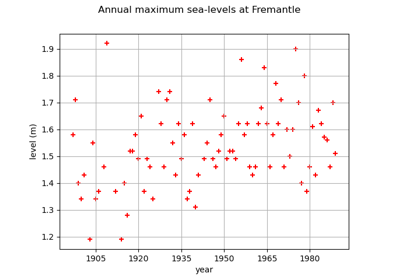
Estimate tail dependence coefficients on the wave-surge data
Estimate tail dependence coefficients on the wind data
Create the distribution of the maximum of independent distributions
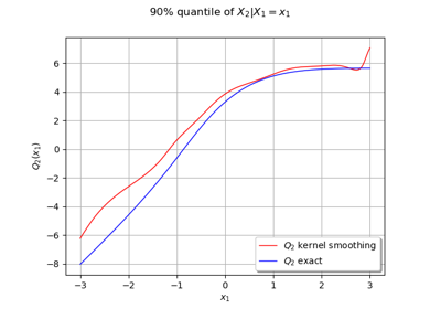
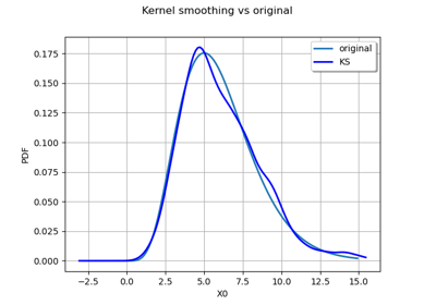
Create your own distribution given its quantile function

Create a gaussian process from a cov. model using HMatrix


Create a process from random vectors and processes
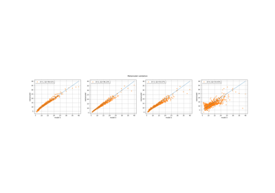
Sample trajectories from a Gaussian Process with correlated outputs
Create a polynomial chaos metamodel by integration on the cantilever beam
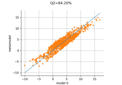
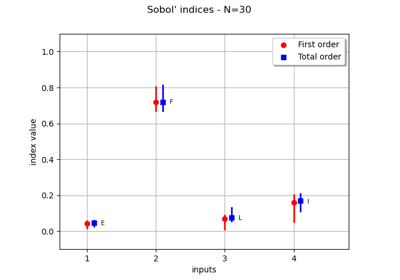
Create a polynomial chaos for the Ishigami function: a quick start guide to polynomial chaos
Example of multi output Kriging on the fire satellite model
Kriging: choose a polynomial trend on the beam model
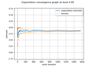
Evaluate the mean of a random vector by simulations
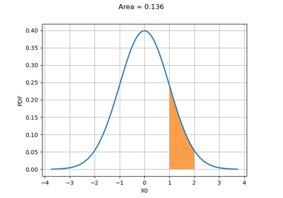
Estimate a probability with Monte-Carlo on axial stressed beam: a quick start guide to reliability
Use the FORM algorithm in case of several design points
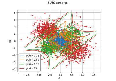
Non parametric Adaptive Importance Sampling (NAIS)

Axial stressed beam : comparing different methods to estimate a probability
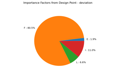
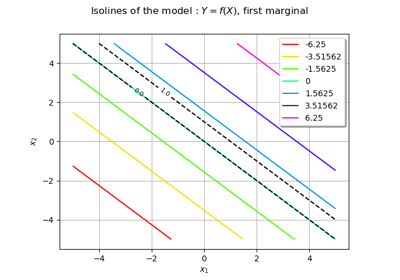
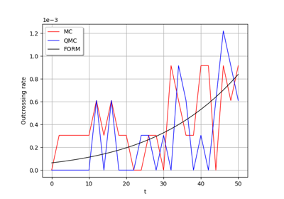
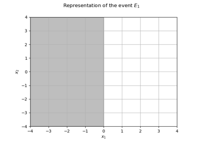
An illustrated example of a FORM probability estimate
Estimate Sobol indices on a field to point function
Estimate Sobol’ indices for a function with multivariate output
Example of sensitivity analyses on the wing weight model
Create mixed deterministic and probabilistic designs of experiments
Create a design of experiments with discrete and continuous variables
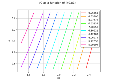
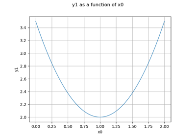
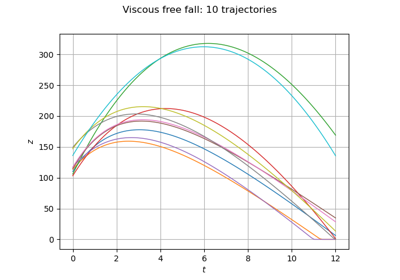
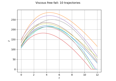
Define a function with a field output: the viscous free fall example
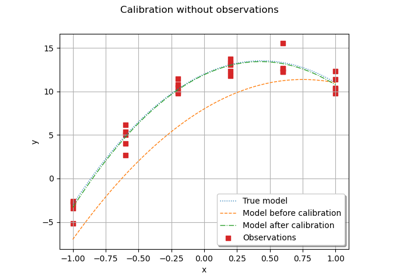
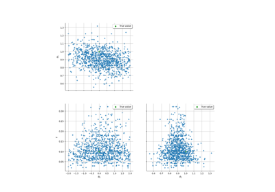
Calibrate a parametric model: a quick-start guide to calibration
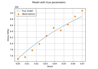
Generate observations of the Chaboche mechanical model
Linear Regression with interval-censored observations
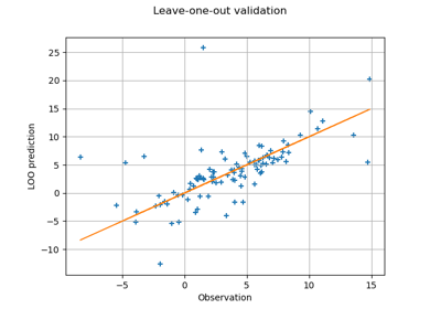
Compute leave-one-out error of a polynomial chaos expansion
Compute confidence intervals of a regression model from data
Compute confidence intervals of a univariate noisy function
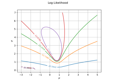
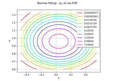
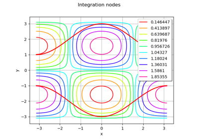
Plot the log-likelihood contours of a distribution