ComposedDistribution distribution
(Source code, png)

- class ComposedDistribution(*args)
Composed distribution.
- Available constructors:
ComposedDistribution(distributions, copula=ot.IndependentCopula(n))
- Parameters:
- distributionslist of
Distribution List of
 marginals of the distribution. Each marginal must be of
dimension 1.
marginals of the distribution. Each marginal must be of
dimension 1.- copula
Distribution A copula. If not mentioned, the copula is set to an
IndependentCopulawith the same dimension as distributions.
- distributionslist of
See also
Notes
A ComposedDistribution is a
-dimensional distribution which can be
written in terms of 1-d marginal distribution functions and a copula  which describes the dependence structure between the variables.
Its cumulative distribution function
which describes the dependence structure between the variables.
Its cumulative distribution function  is defined by its marginal
distributions
is defined by its marginal
distributions  and the copula through the relation:
Examples
>>> import openturns as ot
>>> copula = ot.GumbelCopula(2.0)
>>> marginals = [ot.Uniform(1.0, 2.0), ot.Normal(2.0, 3.0)]
>>> distribution = ot.ComposedDistribution(marginals, copula)
Draw a sample:
>>> sample = distribution.getSample(5)
Methods
abs()Transform distribution by absolute value function.
acos()Transform distribution by arccosine function.
acosh()Transform distribution by acosh function.
asin()Transform distribution by arcsine function.
asinh()Transform distribution by asinh function.
atan()Transform distribution by arctangent function.
atanh()Transform distribution by atanh function.
cbrt()Transform distribution by cubic root function.
Compute a bilateral confidence interval.
computeBilateralConfidenceIntervalWithMarginalProbability(prob)Compute a bilateral confidence interval.
computeCDF(*args)Compute the cumulative distribution function.
computeCDFGradient(*args)Compute the gradient of the cumulative distribution function.
Compute the characteristic function.
computeComplementaryCDF(*args)Compute the complementary cumulative distribution function.
computeConditionalCDF(*args)Compute the conditional cumulative distribution function.
computeConditionalDDF(x, y)Compute the conditional derivative density function of the last component.
computeConditionalPDF(*args)Compute the conditional probability density function.
computeConditionalQuantile(*args)Compute the conditional quantile function of the last component.
computeDDF(*args)Compute the derivative density function.
Compute the entropy of the distribution.
computeGeneratingFunction(*args)Compute the probability-generating function.
Compute the inverse survival function.
Compute the logarithm of the characteristic function.
computeLogGeneratingFunction(*args)Compute the logarithm of the probability-generating function.
computeLogPDF(*args)Compute the logarithm of the probability density function.
computeLogPDFGradient(*args)Compute the gradient of the log probability density function.
Compute the lower extremal dependence coefficients.
Compute the lower tail dependence coefficients.
Compute the confidence interval with minimum volume.
Compute the confidence interval with minimum volume.
Compute the confidence domain with minimum volume.
Compute the confidence domain with minimum volume.
computePDF(*args)Compute the probability density function.
computePDFGradient(*args)Compute the gradient of the probability density function.
computeProbability(interval)Compute the interval probability.
computeQuantile(*args)Compute the quantile function.
computeRadialDistributionCDF(radius[, tail])Compute the cumulative distribution function of the squared radius.
computeScalarQuantile(prob[, tail])Compute the quantile function for univariate distributions.
Compute the sequential conditional cumulative distribution functions.
Compute the sequential conditional derivative density function.
Compute the sequential conditional probability density function.
Compute the conditional quantile function of the last component.
computeSurvivalFunction(*args)Compute the survival function.
computeUnilateralConfidenceInterval(prob[, tail])Compute a unilateral confidence interval.
computeUnilateralConfidenceIntervalWithMarginalProbability(...)Compute a unilateral confidence interval.
Compute the upper extremal dependence coefficients.
Compute the upper tail dependence coefficients.
cos()Transform distribution by cosine function.
cosh()Transform distribution by cosh function.
drawCDF(*args)Draw the cumulative distribution function.
drawLogPDF(*args)Draw the graph or of iso-lines of log-probability density function.
Draw the lower extremal dependence function.
Draw the lower tail dependence function.
drawMarginal1DCDF(marginalIndex, xMin, xMax, ...)Draw the cumulative distribution function of a margin.
drawMarginal1DLogPDF(marginalIndex, xMin, ...)Draw the log-probability density function of a margin.
drawMarginal1DPDF(marginalIndex, xMin, xMax, ...)Draw the probability density function of a margin.
drawMarginal1DSurvivalFunction(...[, logScale])Draw the cumulative distribution function of a margin.
drawMarginal2DCDF(firstMarginal, ...[, ...])Draw the cumulative distribution function of a couple of margins.
drawMarginal2DLogPDF(firstMarginal, ...[, ...])Draw the log-probability density function of a couple of margins.
drawMarginal2DPDF(firstMarginal, ...[, ...])Draw the probability density function of a couple of margins.
drawMarginal2DSurvivalFunction(...[, ...])Draw the cumulative distribution function of a couple of margins.
drawPDF(*args)Draw the graph or of iso-lines of probability density function.
drawQuantile(*args)Draw the quantile function.
drawSurvivalFunction(*args)Draw the cumulative distribution function.
Draw the upper extremal dependence function.
Draw the upper tail dependence function.
exp()Transform distribution by exponential function.
Accessor to the CDF computation precision.
Accessor to the componentwise central moments.
Accessor to the Cholesky factor of the covariance matrix.
Accessor to the object's name.
Accessor to the copula of the distribution.
Accessor to the correlation matrix.
Accessor to the covariance matrix.
Accessor to the componentwise description.
Accessor to the dimension of the distribution.
Dispersion indicator accessor.
Get the marginals of the distribution.
getId()Accessor to the object's id.
Accessor to the number of Gauss integration points.
Accessor to the inverse Cholesky factor of the covariance matrix.
Accessor to the inverse iso-probabilistic transformation.
Accessor to the iso-probabilistic transformation.
Accessor to the Kendall coefficients matrix.
Accessor to the componentwise kurtosis.
getMarginal(*args)Accessor to marginal distributions.
getMean()Accessor to the mean.
getMoment(n)Accessor to the componentwise moments.
getName()Accessor to the object's name.
Accessor to the PDF computation precision.
Accessor to the parameter of the distribution.
Accessor to the parameter description of the distribution.
Accessor to the number of parameters in the distribution.
Accessor to the parameter of the distribution.
Accessor to the Pearson correlation matrix.
Position indicator accessor.
Accessor to the discrete probability levels.
getRange()Accessor to the range of the distribution.
Accessor to a pseudo-random realization from the distribution.
Accessor to roughness of the distribution.
getSample(size)Accessor to a pseudo-random sample from the distribution.
getSampleByInversion(size)Accessor to a pseudo-random sample from the distribution.
getSampleByQMC(size)Accessor to a low discrepancy sample from the distribution.
Accessor to the object's shadowed id.
Accessor to the shape matrix of the underlying copula if it is elliptical.
getShiftedMoment(n, shift)Accessor to the componentwise shifted moments.
Accessor to the singularities of the PDF function.
Accessor to the componentwise skewness.
Accessor to the Spearman correlation matrix.
Accessor to the componentwise standard deviation.
Accessor to the standard distribution.
Accessor to the standard representative distribution in the parametric family.
getSupport(*args)Accessor to the support of the distribution.
Accessor to the object's visibility state.
Test whether the copula of the distribution is elliptical or not.
Test whether the copula of the distribution is the independent one.
hasName()Test if the object is named.
Test if the object has a distinguishable name.
inverse()Transform distribution by inverse function.
Test whether the distribution is continuous or not.
isCopula()Test whether the distribution is a copula or not.
Test whether the distribution is discrete or not.
Test whether the distribution is elliptical or not.
Test whether the distribution is integer-valued or not.
ln()Transform distribution by natural logarithm function.
log()Transform distribution by natural logarithm function.
setCopula(copula)Set the copula of the distribution.
setDescription(description)Accessor to the componentwise description.
Set the marginals of the distribution.
setIntegrationNodesNumber(integrationNodesNumber)Accessor to the number of Gauss integration points.
setName(name)Accessor to the object's name.
setParameter(parameter)Accessor to the parameter of the distribution.
setParametersCollection(*args)Accessor to the parameter of the distribution.
setShadowedId(id)Accessor to the object's shadowed id.
setVisibility(visible)Accessor to the object's visibility state.
sin()Transform distribution by sine function.
sinh()Transform distribution by sinh function.
sqr()Transform distribution by square function.
sqrt()Transform distribution by square root function.
tan()Transform distribution by tangent function.
tanh()Transform distribution by tanh function.
computeDensityGenerator
computeDensityGeneratorDerivative
computeDensityGeneratorSecondDerivative
- __init__(*args)
- abs()
Transform distribution by absolute value function.
- Returns:
- dist
Distribution The transformed distribution.
- dist
- acos()
Transform distribution by arccosine function.
- Returns:
- dist
Distribution The transformed distribution.
- dist
- acosh()
Transform distribution by acosh function.
- Returns:
- dist
Distribution The transformed distribution.
- dist
- asin()
Transform distribution by arcsine function.
- Returns:
- dist
Distribution The transformed distribution.
- dist
- asinh()
Transform distribution by asinh function.
- Returns:
- dist
Distribution The transformed distribution.
- dist
- atan()
Transform distribution by arctangent function.
- Returns:
- dist
Distribution The transformed distribution.
- dist
- atanh()
Transform distribution by atanh function.
- Returns:
- dist
Distribution The transformed distribution.
- dist
- cbrt()
Transform distribution by cubic root function.
- Returns:
- dist
Distribution The transformed distribution.
- dist
- computeBilateralConfidenceInterval(prob)
Compute a bilateral confidence interval.
- Parameters:
- alphafloat,
![\alpha \in [0,1]](data:image/svg+xml;base64,PD94bWwgdmVyc2lvbj0nMS4wJyBlbmNvZGluZz0nVVRGLTgnPz4KPCEtLSBUaGlzIGZpbGUgd2FzIGdlbmVyYXRlZCBieSBkdmlzdmdtIDMuMiAtLT4KPHN2ZyB2ZXJzaW9uPScxLjEnIHhtbG5zPSdodHRwOi8vd3d3LnczLm9yZy8yMDAwL3N2ZycgeG1sbnM6eGxpbms9J2h0dHA6Ly93d3cudzMub3JnLzE5OTkveGxpbmsnIHdpZHRoPSc0NS41ODY5ODNwdCcgaGVpZ2h0PScxMS45NTUxNjhwdCcgdmlld0JveD0nMCAtOC45NjYzNzYgNDUuNTg2OTgzIDExLjk1NTE2OCc+CjxkZWZzPgo8cGF0aCBpZD0nZzItNDgnIGQ9J001LjM1NTkxNS0zLjgyNTY1NEM1LjM1NTkxNS00LjgxNzkzMyA1LjI5NjEzOS01Ljc4NjMwMSA0Ljg2NTc1My02LjY5NDg5NEM0LjM3NTU5Mi03LjY4NzE3MyAzLjUxNDgxOS03Ljk1MDE4NyAyLjkyOTAxNi03Ljk1MDE4N0MyLjIzNTYxNi03Ljk1MDE4NyAxLjM4NjgtNy42MDM0ODcgLjk0NDQ1OC02LjYxMTIwOEMuNjA5NzE0LTUuODU4MDMyIC40OTAxNjItNS4xMTY4MTIgLjQ5MDE2Mi0zLjgyNTY1NEMuNDkwMTYyLTIuNjY2MDAyIC41NzM4NDgtMS43OTMyNzUgMS4wMDQyMzQtLjk0NDQ1OEMxLjQ3MDQ4Ni0uMDM1ODY2IDIuMjk1MzkyIC4yNTEwNTkgMi45MTcwNjEgLjI1MTA1OUMzLjk1NzE2MSAuMjUxMDU5IDQuNTU0OTE5LS4zNzA2MSA0LjkwMTYxOS0xLjA2NDAxQzUuMzMyMDA1LTEuOTYwNjQ4IDUuMzU1OTE1LTMuMTMyMjU0IDUuMzU1OTE1LTMuODI1NjU0Wk0yLjkxNzA2MSAuMDExOTU1QzIuNTM0NDk2IC4wMTE5NTUgMS43NTc0MS0uMjAzMjM4IDEuNTMwMjYyLTEuNTA2MzUxQzEuMzk4NzU1LTIuMjIzNjYxIDEuMzk4NzU1LTMuMTMyMjU0IDEuMzk4NzU1LTMuOTY5MTE2QzEuMzk4NzU1LTQuOTQ5NDQgMS4zOTg3NTUtNS44MzQxMjIgMS41OTAwMzctNi41Mzk0NzdDMS43OTMyNzUtNy4zNDA0NzMgMi40MDI5ODktNy43MTEwODMgMi45MTcwNjEtNy43MTEwODNDMy4zNzEzNTctNy43MTEwODMgNC4wNjQ3NTctNy40MzYxMTUgNC4yOTE5MDUtNi40MDc5N0M0LjQ0NzMyMy01LjcyNjUyNiA0LjQ0NzMyMy00Ljc4MjA2NyA0LjQ0NzMyMy0zLjk2OTExNkM0LjQ0NzMyMy0zLjE2ODEyIDQuNDQ3MzIzLTIuMjU5NTI3IDQuMzE1ODE2LTEuNTMwMjYyQzQuMDg4NjY3LS4yMTUxOTMgMy4zMzU0OTIgLjAxMTk1NSAyLjkxNzA2MSAuMDExOTU1WicvPgo8cGF0aCBpZD0nZzItNDknIGQ9J00zLjQ0MzA4OC03LjY2MzI2M0MzLjQ0MzA4OC03LjkzODIzMiAzLjQ0MzA4OC03Ljk1MDE4NyAzLjIwMzk4NS03Ljk1MDE4N0MyLjkxNzA2MS03LjYyNzM5NyAyLjMxOTMwMy03LjE4NTA1NiAxLjA4NzkyLTcuMTg1MDU2Vi02LjgzODM1NkMxLjM2Mjg4OS02LjgzODM1NiAxLjk2MDY0OC02LjgzODM1NiAyLjYxODE4Mi03LjE0OTE5MVYtLjkyMDU0OEMyLjYxODE4Mi0uNDkwMTYyIDIuNTgyMzE2LS4zNDY3IDEuNTMwMjYyLS4zNDY3SDEuMTU5NjUxVjBDMS40ODI0NDEtLjAyMzkxIDIuNjQyMDkyLS4wMjM5MSAzLjAzNjYxMy0uMDIzOTFTNC41Nzg4MjktLjAyMzkxIDQuOTAxNjE5IDBWLS4zNDY3SDQuNTMxMDA5QzMuNDc4OTU0LS4zNDY3IDMuNDQzMDg4LS40OTAxNjIgMy40NDMwODgtLjkyMDU0OFYtNy42NjMyNjNaJy8+CjxwYXRoIGlkPSdnMi05MScgZD0nTTIuOTg4NzkyIDIuOTg4NzkyVjIuNTQ2NDUxSDEuODI5MTQxVi04LjUyNDAzNUgyLjk4ODc5MlYtOC45NjYzNzZIMS4zODY4VjIuOTg4NzkySDIuOTg4NzkyWicvPgo8cGF0aCBpZD0nZzItOTMnIGQ9J00xLjg1MzA1MS04Ljk2NjM3NkguMjUxMDU5Vi04LjUyNDAzNUgxLjQxMDcxVjIuNTQ2NDUxSC4yNTEwNTlWMi45ODg3OTJIMS44NTMwNTFWLTguOTY2Mzc2WicvPgo8cGF0aCBpZD0nZzAtNTAnIGQ9J002LjU1MTQzMi0yLjc0OTY4OUM2Ljc1NDY3LTIuNzQ5Njg5IDYuOTY5ODYzLTIuNzQ5Njg5IDYuOTY5ODYzLTIuOTg4NzkyUzYuNzU0NjctMy4yMjc4OTUgNi41NTE0MzItMy4yMjc4OTVIMS40ODI0NDFDMS42MjU5MDMtNC44Mjk4ODggMy4wMDA3NDctNS45Nzc1ODQgNC42ODY0MjYtNS45Nzc1ODRINi41NTE0MzJDNi43NTQ2Ny01Ljk3NzU4NCA2Ljk2OTg2My01Ljk3NzU4NCA2Ljk2OTg2My02LjIxNjY4N1M2Ljc1NDY3LTYuNDU1NzkxIDYuNTUxNDMyLTYuNDU1NzkxSDQuNjYyNTE2QzIuNjE4MTgyLTYuNDU1NzkxIC45OTIyNzktNC45MDE2MTkgLjk5MjI3OS0yLjk4ODc5MlMyLjYxODE4MiAuNDc4MjA3IDQuNjYyNTE2IC40NzgyMDdINi41NTE0MzJDNi43NTQ2NyAuNDc4MjA3IDYuOTY5ODYzIC40NzgyMDcgNi45Njk4NjMgLjIzOTEwM1M2Ljc1NDY3IDAgNi41NTE0MzIgMEg0LjY4NjQyNkMzLjAwMDc0NyAwIDEuNjI1OTAzLTEuMTQ3Njk2IDEuNDgyNDQxLTIuNzQ5Njg5SDYuNTUxNDMyWicvPgo8cGF0aCBpZD0nZzEtMTEnIGQ9J001LjUzNTI0My0zLjAyNDY1OEM1LjUzNTI0My00LjE4NDMwOSA0Ljg3NzcwOS01LjI3MjIyOSAzLjYxMDQ2MS01LjI3MjIyOUMyLjA0NDMzNC01LjI3MjIyOSAuNDc4MjA3LTMuNTYyNjQgLjQ3ODIwNy0xLjg2NTAwNkMuNDc4MjA3LS44MjQ5MDcgMS4xMjM3ODYgLjExOTU1MiAyLjM0MzIxMyAuMTE5NTUyQzMuMDg0NDMzIC4xMTk1NTIgMy45NjkxMTYtLjE2NzM3MiA0LjgxNzkzMy0uODg0NjgyQzQuOTg1MzA1LS4yMTUxOTMgNS4zNTU5MTUgLjExOTU1MiA1Ljg2OTk4OCAuMTE5NTUyQzYuNTE1NTY3IC4xMTk1NTIgNi44MzgzNTYtLjU0OTkzOCA2LjgzODM1Ni0uNzA1MzU1QzYuODM4MzU2LS44MTI5NTEgNi43NTQ2Ny0uODEyOTUxIDYuNzE4ODA0LS44MTI5NTFDNi42MjMxNjMtLjgxMjk1MSA2LjYxMTIwOC0uNzc3MDg2IDYuNTc1MzQyLS42ODE0NDVDNi40Njc3NDYtLjM4MjU2NSA2LjE5Mjc3Ny0uMTE5NTUyIDUuOTA1ODUzLS4xMTk1NTJDNS41MzUyNDMtLjExOTU1MiA1LjUzNTI0My0uODg0NjgyIDUuNTM1MjQzLTEuNjEzOTQ4QzYuNzU0NjctMy4wNzI0NzggNy4wNDE1OTQtNC41Nzg4MjkgNy4wNDE1OTQtNC41OTA3ODVDNy4wNDE1OTQtNC42OTgzODEgNi45NDU5NTMtNC42OTgzODEgNi45MTAwODctNC42OTgzODFDNi44MDI0OTEtNC42OTgzODEgNi43OTA1MzUtNC42NjI1MTYgNi43NDI3MTUtNC40NDczMjNDNi41ODcyOTgtMy45MjEyOTUgNi4yNzY0NjMtMi45ODg3OTIgNS41MzUyNDMtMi4wMDg0NjhWLTMuMDI0NjU4Wk00Ljc4MjA2Ny0xLjE3MTYwNkMzLjczMDAxMi0uMjI3MTQ4IDIuNzg1NTU0LS4xMTk1NTIgMi4zNjcxMjMtLjExOTU1MkMxLjUxODMwNi0uMTE5NTUyIDEuMjc5MjAzLS44NzI3MjcgMS4yNzkyMDMtMS40MzQ2MkMxLjI3OTIwMy0xLjk0ODY5MiAxLjU0MjIxNy0zLjE2ODEyIDEuOTEyODI3LTMuODI1NjU0QzIuNDAyOTg5LTQuNjYyNTE2IDMuMDcyNDc4LTUuMDMzMTI2IDMuNjEwNDYxLTUuMDMzMTI2QzQuNzcwMTEyLTUuMDMzMTI2IDQuNzcwMTEyLTMuNTE0ODE5IDQuNzcwMTEyLTIuNTEwNTg1QzQuNzcwMTEyLTIuMjExNzA2IDQuNzU4MTU3LTEuOTAwODcyIDQuNzU4MTU3LTEuNjAxOTkzQzQuNzU4MTU3LTEuMzYyODg5IDQuNzcwMTEyLTEuMzAzMTEzIDQuNzgyMDY3LTEuMTcxNjA2WicvPgo8cGF0aCBpZD0nZzEtNTknIGQ9J00yLjMzMTI1OCAuMDQ3ODIxQzIuMzMxMjU4LS42NDU1NzkgMi4xMDQxMS0xLjE1OTY1MSAxLjYxMzk0OC0xLjE1OTY1MUMxLjIzMTM4Mi0xLjE1OTY1MSAxLjA0MDEtLjg0ODgxNyAxLjA0MDEtLjU4NTgwM1MxLjIxOTQyNyAwIDEuNjI1OTAzIDBDMS43ODEzMiAwIDEuOTEyODI3LS4wNDc4MjEgMi4wMjA0MjMtLjE1NTQxN0MyLjA0NDMzNC0uMTc5MzI4IDIuMDU2Mjg5LS4xNzkzMjggMi4wNjgyNDQtLjE3OTMyOEMyLjA5MjE1NC0uMTc5MzI4IDIuMDkyMTU0LS4wMTE5NTUgMi4wOTIxNTQgLjA0NzgyMUMyLjA5MjE1NCAuNDQyMzQxIDIuMDIwNDIzIDEuMjE5NDI3IDEuMzI3MDI0IDEuOTk2NTEzQzEuMTk1NTE3IDIuMTM5OTc1IDEuMTk1NTE3IDIuMTYzODg1IDEuMTk1NTE3IDIuMTg3Nzk2QzEuMTk1NTE3IDIuMjQ3NTcyIDEuMjU1MjkzIDIuMzA3MzQ3IDEuMzE1MDY4IDIuMzA3MzQ3QzEuNDEwNzEgMi4zMDczNDcgMi4zMzEyNTggMS40MjI2NjUgMi4zMzEyNTggLjA0NzgyMVonLz4KPC9kZWZzPgo8ZyBpZD0ncGFnZTEnPgo8dXNlIHg9JzAnIHk9JzAnIHhsaW5rOmhyZWY9JyNnMS0xMScvPgo8dXNlIHg9JzEwLjg0MjU1MycgeT0nMCcgeGxpbms6aHJlZj0nI2cwLTUwJy8+Cjx1c2UgeD0nMjIuMTMzNTIyJyB5PScwJyB4bGluazpocmVmPScjZzItOTEnLz4KPHVzZSB4PScyNS4zODUxODMnIHk9JzAnIHhsaW5rOmhyZWY9JyNnMi00OCcvPgo8dXNlIHg9JzMxLjIzODE3MycgeT0nMCcgeGxpbms6aHJlZj0nI2cxLTU5Jy8+Cjx1c2UgeD0nMzYuNDgyMzMyJyB5PScwJyB4bGluazpocmVmPScjZzItNDknLz4KPHVzZSB4PSc0Mi4zMzUzMjInIHk9JzAnIHhsaW5rOmhyZWY9JyNnMi05MycvPgo8L2c+Cjwvc3ZnPgo8IS0tIERFUFRIPTQgLS0+)
The confidence level.
- alphafloat,
- Returns:
- confInterval
Interval The confidence interval of level
 .
.
- confInterval
Notes
We consider an absolutely continuous measure
 with density function
  .
.The bilateral confidence interval
 is the cartesian product
 ![I^*_{\alpha} = [a_1, b_1] \times \dots \times [a_d, b_d]](data:image/svg+xml;base64,PD94bWwgdmVyc2lvbj0nMS4wJyBlbmNvZGluZz0nVVRGLTgnPz4KPCEtLSBUaGlzIGZpbGUgd2FzIGdlbmVyYXRlZCBieSBkdmlzdmdtIDMuMiAtLT4KPHN2ZyB2ZXJzaW9uPScxLjEnIHhtbG5zPSdodHRwOi8vd3d3LnczLm9yZy8yMDAwL3N2ZycgeG1sbnM6eGxpbms9J2h0dHA6Ly93d3cudzMub3JnLzE5OTkveGxpbmsnIHdpZHRoPScxMzQuOTMyMTg3cHQnIGhlaWdodD0nMTEuOTU1MTY4cHQnIHZpZXdCb3g9JzAgLTguOTY2Mzc2IDEzNC45MzIxODcgMTEuOTU1MTY4Jz4KPGRlZnM+CjxwYXRoIGlkPSdnNC00OScgZD0nTTIuNTAyNjE1LTUuMDc2OTYxQzIuNTAyNjE1LTUuMjkyMTU0IDIuNDg2Njc1LTUuMzAwMTI1IDIuMjcxNDgyLTUuMzAwMTI1QzEuOTQ0NzA3LTQuOTgxMzIgMS41MjIyOTEtNC43OTAwMzcgLjc2NTEzMS00Ljc5MDAzN1YtNC41MjcwMjRDLjk4MDMyNC00LjUyNzAyNCAxLjQxMDcxLTQuNTI3MDI0IDEuODcyOTc2LTQuNzQyMjE3Vi0uNjUzNTQ5QzEuODcyOTc2LS4zNTg2NTUgMS44NDkwNjYtLjI2MzAxNCAxLjA5MTkwNS0uMjYzMDE0SC44MTI5NTFWMEMxLjEzOTcyNi0uMDIzOTEgMS44MjUxNTYtLjAyMzkxIDIuMTgzODExLS4wMjM5MVMzLjIzNTg2Ni0uMDIzOTEgMy41NjI2NCAwVi0uMjYzMDE0SDMuMjgzNjg2QzIuNTI2NTI2LS4yNjMwMTQgMi41MDI2MTUtLjM1ODY1NSAyLjUwMjYxNS0uNjUzNTQ5Vi01LjA3Njk2MVonLz4KPHBhdGggaWQ9J2c1LTYxJyBkPSdNOC4wNjk3MzgtMy44NzM0NzRDOC4yMzcxMTEtMy44NzM0NzQgOC40NTIzMDQtMy44NzM0NzQgOC40NTIzMDQtNC4wODg2NjdDOC40NTIzMDQtNC4zMTU4MTYgOC4yNDkwNjYtNC4zMTU4MTYgOC4wNjk3MzgtNC4zMTU4MTZIMS4wMjgxNDRDLjg2MDc3Mi00LjMxNTgxNiAuNjQ1NTc5LTQuMzE1ODE2IC42NDU1NzktNC4xMDA2MjNDLjY0NTU3OS0zLjg3MzQ3NCAuODQ4ODE3LTMuODczNDc0IDEuMDI4MTQ0LTMuODczNDc0SDguMDY5NzM4Wk04LjA2OTczOC0xLjY0OTgxM0M4LjIzNzExMS0xLjY0OTgxMyA4LjQ1MjMwNC0xLjY0OTgxMyA4LjQ1MjMwNC0xLjg2NTAwNkM4LjQ1MjMwNC0yLjA5MjE1NCA4LjI0OTA2Ni0yLjA5MjE1NCA4LjA2OTczOC0yLjA5MjE1NEgxLjAyODE0NEMuODYwNzcyLTIuMDkyMTU0IC42NDU1NzktMi4wOTIxNTQgLjY0NTU3OS0xLjg3Njk2MUMuNjQ1NTc5LTEuNjQ5ODEzIC44NDg4MTctMS42NDk4MTMgMS4wMjgxNDQtMS42NDk4MTNIOC4wNjk3MzhaJy8+CjxwYXRoIGlkPSdnNS05MScgZD0nTTIuOTg4NzkyIDIuOTg4NzkyVjIuNTQ2NDUxSDEuODI5MTQxVi04LjUyNDAzNUgyLjk4ODc5MlYtOC45NjYzNzZIMS4zODY4VjIuOTg4NzkySDIuOTg4NzkyWicvPgo8cGF0aCBpZD0nZzUtOTMnIGQ9J00xLjg1MzA1MS04Ljk2NjM3NkguMjUxMDU5Vi04LjUyNDAzNUgxLjQxMDcxVjIuNTQ2NDUxSC4yNTEwNTlWMi45ODg3OTJIMS44NTMwNTFWLTguOTY2Mzc2WicvPgo8cGF0aCBpZD0nZzEtMScgZD0nTTIuMjk1MzkyLTIuOTg4NzkyQzIuMjk1MzkyLTMuMzM1NDkyIDIuMDA4NDY4LTMuNjIyNDE2IDEuNjYxNzY4LTMuNjIyNDE2UzEuMDI4MTQ0LTMuMzM1NDkyIDEuMDI4MTQ0LTIuOTg4NzkyUzEuMzE1MDY4LTIuMzU1MTY4IDEuNjYxNzY4LTIuMzU1MTY4UzIuMjk1MzkyLTIuNjQyMDkyIDIuMjk1MzkyLTIuOTg4NzkyWicvPgo8cGF0aCBpZD0nZzEtMicgZD0nTTQuNjUwNTYtMy4zMjM1MzdMMi4yNTk1MjctNS43MDI2MTVDMi4xMTYwNjUtNS44NDYwNzcgMi4wOTIxNTQtNS44Njk5ODggMS45OTY1MTMtNS44Njk5ODhDMS44NzY5NjEtNS44Njk5ODggMS43NTc0MS01Ljc2MjM5MSAxLjc1NzQxLTUuNjMwODg0QzEuNzU3NDEtNS41NDcxOTggMS43ODEzMi01LjUyMzI4OCAxLjkxMjgyNy01LjM5MTc4MUw0LjMwMzg2MS0yLjk4ODc5MkwxLjkxMjgyNy0uNTg1ODAzQzEuNzgxMzItLjQ1NDI5NiAxLjc1NzQxLS40MzAzODYgMS43NTc0MS0uMzQ2N0MxLjc1NzQxLS4yMTUxOTMgMS44NzY5NjEtLjEwNzU5NyAxLjk5NjUxMy0uMTA3NTk3QzIuMDkyMTU0LS4xMDc1OTcgMi4xMTYwNjUtLjEzMTUwNyAyLjI1OTUyNy0uMjc0OTY5TDQuNjM4NjA1LTIuNjU0MDQ3TDcuMTEzMzI1LS4xNzkzMjhDNy4xMzcyMzUtLjE2NzM3MiA3LjIyMDkyMi0uMTA3NTk3IDcuMjkyNjUzLS4xMDc1OTdDNy40MzYxMTUtLjEwNzU5NyA3LjUzMTc1Ni0uMjE1MTkzIDcuNTMxNzU2LS4zNDY3QzcuNTMxNzU2LS4zNzA2MSA3LjUzMTc1Ni0uNDE4NDMxIDcuNDk1ODktLjQ3ODIwN0M3LjQ4MzkzNS0uNTAyMTE3IDUuNTgzMDY0LTIuMzc5MDc4IDQuOTg1MzA1LTIuOTg4NzkyTDcuMTczMTAxLTUuMTc2NTg4QzcuMjMyODc3LTUuMjQ4MzE5IDcuNDEyMjA0LTUuNDAzNzM2IDcuNDcxOTgtNS40NzU0NjdDNy40ODM5MzUtNS40OTkzNzcgNy41MzE3NTYtNS41NDcxOTggNy41MzE3NTYtNS42MzA4ODRDNy41MzE3NTYtNS43NjIzOTEgNy40MzYxMTUtNS44Njk5ODggNy4yOTI2NTMtNS44Njk5ODhDNy4xOTcwMTEtNS44Njk5ODggNy4xNDkxOTEtNS44MjIxNjcgNy4wMTc2ODQtNS42OTA2Nkw0LjY1MDU2LTMuMzIzNTM3WicvPgo8cGF0aCBpZD0nZzItMTEnIGQ9J000LjA2NDc1Ny0xLjExNTgxNkM0LjgwNTk3OC0xLjkyODc2NyA1LjA2ODk5MS0yLjk2NDg4MiA1LjA2ODk5MS0zLjAyODY0M0M1LjA2ODk5MS0zLjEwMDM3NCA1LjAyMTE3MS0zLjEzMjI1NCA0Ljk0OTQ0LTMuMTMyMjU0QzQuODQ1ODI4LTMuMTMyMjU0IDQuODM3ODU4LTMuMTAwMzc0IDQuNzkwMDM3LTIuOTMzMDAxQzQuNTY2ODc0LTIuMTIwMDUgNC4wODg2NjctMS40OTgzODEgNC4wNjQ3NTctMS40OTgzODFDNC4wNDg4MTctMS40OTgzODEgNC4wNDg4MTctMS42OTc2MzQgNC4wNDg4MTctMS44MjUxNTZDNC4wMzI4NzctMy4yMjc4OTUgMy4xMjQyODQtMy41MTQ4MTkgMi41ODIzMTYtMy41MTQ4MTlDMS40NTg1MzEtMy41MTQ4MTkgLjM1MDY4NS0yLjQyMjkxNCAuMzUwNjg1LTEuMjk5MTI4Qy4zNTA2ODUtLjUxMDA4NyAuOTAwNjIzIC4wNzk3MDEgMS43NDU0NTUgLjA3OTcwMUMyLjMwMzM2MiAuMDc5NzAxIDIuODkzMTUxLS4xMTk1NTIgMy41MjI3OS0uNTg5Nzg4QzMuNjk4MTMyIC4wMzk4NTEgNC4xNjAzOTkgLjA3OTcwMSA0LjMwMzg2MSAuMDc5NzAxQzQuNzU4MTU3IC4wNzk3MDEgNS4wMjExNzEtLjMyNjc3NSA1LjAyMTE3MS0uNDc4MjA3QzUuMDIxMTcxLS41NzM4NDggNC45MjU1MjktLjU3Mzg0OCA0LjkwMTYxOS0uNTczODQ4QzQuODEzOTQ4LS41NzM4NDggNC43OTgwMDctLjU0OTkzOCA0Ljc3NDA5Ny0uNDk0MTQ3QzQuNjQ2NTc1LS4xNTk0MDIgNC4zNzU1OTItLjE0MzQ2MiA0LjMzNTc0MS0uMTQzNDYyQzQuMjI0MTU5LS4xNDM0NjIgNC4wOTY2MzgtLjE0MzQ2MiA0LjA2NDc1Ny0xLjExNTgxNlpNMy40NjY5OTktLjg1MjgwMkMyLjkwMTEyMS0uMzQyNzE1IDIuMjMxNjMxLS4xNDM0NjIgMS43NjkzNjUtLjE0MzQ2MkMxLjM1NDkxOS0uMTQzNDYyIC45OTYyNjQtLjM4MjU2NSAuOTk2MjY0LTEuMDIwMTc0Qy45OTYyNjQtMS4yOTkxMjggMS4xMjM3ODYtMi4xMjAwNSAxLjQ5ODM4MS0yLjY1NDA0N0MxLjgxNzE4Ni0zLjEwMDM3NCAyLjI0NzU3Mi0zLjI5MTY1NiAyLjU3NDM0Ni0zLjI5MTY1NkMzLjAxMjcwMi0zLjI5MTY1NiAzLjI1OTc3Ni0yLjk4MDgyMiAzLjM2MzM4Ny0yLjQ5NDY0NUMzLjQ4MjkzOS0xLjk1MjY3NyAzLjQxOTE3OC0xLjMxNTA2OCAzLjQ2Njk5OS0uODUyODAyWicvPgo8cGF0aCBpZD0nZzItMTAwJyBkPSdNNC4yODc5Mi01LjI5MjE1NEM0LjI5NTg5LTUuMzA4MDk1IDQuMzE5ODAxLTUuNDExNzA2IDQuMzE5ODAxLTUuNDE5Njc2QzQuMzE5ODAxLTUuNDU5NTI3IDQuMjg3OTItNS41MzEyNTggNC4xOTIyNzktNS41MzEyNThDNC4xNjAzOTktNS41MzEyNTggMy45MTMzMjUtNS41MDczNDcgMy43MzAwMTItNS40OTE0MDdMMy4yODM2ODYtNS40NTk1MjdDMy4xMDgzNDQtNS40NDM1ODcgMy4wMjg2NDMtNS40MzU2MTYgMy4wMjg2NDMtNS4yOTIxNTRDMy4wMjg2NDMtNS4xODA1NzMgMy4xNDAyMjQtNS4xODA1NzMgMy4yMzU4NjYtNS4xODA1NzNDMy42MTg0MzEtNS4xODA1NzMgMy42MTg0MzEtNS4xMzI3NTIgMy42MTg0MzEtNS4wNjEwMjFDMy42MTg0MzEtNS4wMTMyIDMuNTU0NjctNC43NTAxODcgMy41MTQ4MTktNC41OTA3ODVMMy4xMjQyODQtMy4wMzY2MTNDMy4wNTI1NTMtMy4xNzIxMDUgMi44MjE0Mi0zLjUxNDgxOSAyLjMzNTI0My0zLjUxNDgxOUMxLjM4NjgtMy41MTQ4MTkgLjM0MjcxNS0yLjQwNjk3NCAuMzQyNzE1LTEuMjI3Mzk3Qy4zNDI3MTUtLjM5ODUwNiAuODc2NzEyIC4wNzk3MDEgMS40OTA0MTEgLjA3OTcwMUMyLjAwMDQ5OCAuMDc5NzAxIDIuNDM4ODU0LS4zMjY3NzUgMi41ODIzMTYtLjQ4NjE3N0MyLjcyNTc3OCAuMDYzNzYxIDMuMjY3NzQ2IC4wNzk3MDEgMy4zNjMzODcgLjA3OTcwMUMzLjczMDAxMiAuMDc5NzAxIDMuOTEzMzI1LS4yMjMxNjMgMy45NzcwODYtLjM1ODY1NUM0LjEzNjQ4OC0uNjQ1NTc5IDQuMjQ4MDctMS4xMDc4NDYgNC4yNDgwNy0xLjEzOTcyNkM0LjI0ODA3LTEuMTg3NTQ3IDQuMjE2MTg5LTEuMjQzMzM3IDQuMTIwNTQ4LTEuMjQzMzM3UzQuMDA4OTY2LTEuMTk1NTE3IDMuOTYxMTQ2LS45OTYyNjRDMy44NDk1NjQtLjU1NzkwOCAzLjY5ODEzMi0uMTQzNDYyIDMuMzg3Mjk4LS4xNDM0NjJDMy4yMDM5ODUtLjE0MzQ2MiAzLjEzMjI1NC0uMjk0ODk0IDMuMTMyMjU0LS41MTgwNTdDMy4xMzIyNTQtLjY2OTQ4OSAzLjE1NjE2NC0uNzU3MTYxIDMuMTgwMDc1LS44NjA3NzJMNC4yODc5Mi01LjI5MjE1NFpNMi41ODIzMTYtLjg2MDc3MkMyLjE4MzgxMS0uMzEwODM0IDEuNzY5MzY1LS4xNDM0NjIgMS41MTQzMjEtLjE0MzQ2MkMxLjE0NzY5Ni0uMTQzNDYyIC45NjQzODQtLjQ3ODIwNyAuOTY0Mzg0LS44OTI2NTNDLjk2NDM4NC0xLjI2NzI0OCAxLjE3OTU3Ny0yLjEyMDA1IDEuMzU0OTE5LTIuNDcwNzM1QzEuNTg2MDUyLTIuOTU2OTEyIDEuOTc2NTg4LTMuMjkxNjU2IDIuMzQzMjEzLTMuMjkxNjU2QzIuODYxMjctMy4yOTE2NTYgMy4wMTI3MDItMi43MDk4MzggMy4wMTI3MDItMi42MTQxOTdDMy4wMTI3MDItMi41ODIzMTYgMi44MTM0NS0xLjgwMTI0NSAyLjc2NTYyOS0xLjU5NDAyMkMyLjY2MjAxNy0xLjIxOTQyNyAyLjY2MjAxNy0xLjIwMzQ4NyAyLjU4MjMxNi0uODYwNzcyWicvPgo8cGF0aCBpZD0nZzAtMycgZD0nTTMuMjkxNjU2LTEuMDUyMDU1QzMuMzYzMzg3LTEuMDA0MjM0IDMuMzg3Mjk4LTEuMDA0MjM0IDMuNDI3MTQ4LTEuMDA0MjM0QzMuNTU0NjctMS4wMDQyMzQgMy42NjYyNTItMS4xMDc4NDYgMy42NjYyNTItMS4yNTEzMDhDMy42NjYyNTItMS40MDI3NCAzLjU4NjU1LTEuNDM0NjIgMy40NjY5OTktMS40OTA0MTFDMi45MzMwMDEtMS43Mzc0ODQgMi43NDE3MTktMS44MjUxNTYgMi4zNTExODMtMS45ODQ1NThMMy4yODM2ODYtMi40MDY5NzRDMy4zNDc0NDctMi40MzA4ODQgMy40OTg4NzktMi41MDI2MTUgMy41NjI2NC0yLjUyNjUyNkMzLjY0MjM0MS0yLjU3NDM0NiAzLjY2NjI1Mi0yLjY1NDA0NyAzLjY2NjI1Mi0yLjcyNTc3OEMzLjY2NjI1Mi0yLjgyMTQyIDMuNjE4NDMxLTIuOTcyODUyIDMuMzc5MzI4LTIuOTcyODUyTDIuMjMxNjMxLTIuMTkxNzgxTDIuMzQzMjEzLTMuMzcxMzU3QzIuMzU5MTUzLTMuNTA2ODQ5IDIuMzQzMjEzLTMuNzA2MTAyIDIuMTEyMDgtMy43MDYxMDJDMS45Njg2MTgtMy43MDYxMDIgMS44NTcwMzYtMy41ODY1NSAxLjg4MDk0Ni0zLjQ3NDk2OVYtMy4zNzkzMjhMMS45OTI1MjgtMi4xOTE3ODFMLjkzMjUwMy0yLjkyNTAzMUMuODYwNzcyLTIuOTcyODUyIC44MzY4NjItMi45NzI4NTIgLjc5NzAxMS0yLjk3Mjg1MkMuNjY5NDg5LTIuOTcyODUyIC41NTc5MDgtMi44NjkyNCAuNTU3OTA4LTIuNzI1Nzc4Qy41NTc5MDgtMi41NzQzNDYgLjYzNzYwOS0yLjU0MjQ2NiAuNzU3MTYxLTIuNDg2Njc1QzEuMjkxMTU4LTIuMjM5NjAxIDEuNDgyNDQxLTIuMTUxOTMgMS44NzI5NzYtMS45OTI1MjhMLjk0MDQ3My0xLjU3MDExMkMuODc2NzEyLTEuNTQ2MjAyIC43MjUyOC0xLjQ3NDQ3MSAuNjYxNTE5LTEuNDUwNTZDLjU4MTgxOC0xLjQwMjc0IC41NTc5MDgtMS4zMjMwMzkgLjU1NzkwOC0xLjI1MTMwOEMuNTU3OTA4LTEuMTA3ODQ2IC42Njk0ODktMS4wMDQyMzQgLjc5NzAxMS0xLjAwNDIzNEMuODYwNzcyLTEuMDA0MjM0IC44NzY3MTItMS4wMDQyMzQgMS4wNzU5NjUtMS4xNDc2OTZMMS45OTI1MjgtMS43ODUzMDVMMS44NzI5NzYtLjUwMjExN0MxLjg3Mjk3Ni0uMzQyNzE1IDIuMDA4NDY4LS4yNzA5ODQgMi4xMTIwOC0uMjcwOTg0UzIuMzUxMTgzLS4zNDI3MTUgMi4zNTExODMtLjUwMjExN0MyLjM1MTE4My0uNTgxODE4IDIuMzE5MzAzLS44MzY4NjIgMi4zMTEzMzMtLjkzMjUwM0MyLjI3OTQ1Mi0xLjIwMzQ4NyAyLjI1NTU0Mi0xLjUwNjM1MSAyLjIzMTYzMS0xLjc4NTMwNUwzLjI5MTY1Ni0xLjA1MjA1NVonLz4KPHBhdGggaWQ9J2czLTU5JyBkPSdNMi4zMzEyNTggLjA0NzgyMUMyLjMzMTI1OC0uNjQ1NTc5IDIuMTA0MTEtMS4xNTk2NTEgMS42MTM5NDgtMS4xNTk2NTFDMS4yMzEzODItMS4xNTk2NTEgMS4wNDAxLS44NDg4MTcgMS4wNDAxLS41ODU4MDNTMS4yMTk0MjcgMCAxLjYyNTkwMyAwQzEuNzgxMzIgMCAxLjkxMjgyNy0uMDQ3ODIxIDIuMDIwNDIzLS4xNTU0MTdDMi4wNDQzMzQtLjE3OTMyOCAyLjA1NjI4OS0uMTc5MzI4IDIuMDY4MjQ0LS4xNzkzMjhDMi4wOTIxNTQtLjE3OTMyOCAyLjA5MjE1NC0uMDExOTU1IDIuMDkyMTU0IC4wNDc4MjFDMi4wOTIxNTQgLjQ0MjM0MSAyLjAyMDQyMyAxLjIxOTQyNyAxLjMyNzAyNCAxLjk5NjUxM0MxLjE5NTUxNyAyLjEzOTk3NSAxLjE5NTUxNyAyLjE2Mzg4NSAxLjE5NTUxNyAyLjE4Nzc5NkMxLjE5NTUxNyAyLjI0NzU3MiAxLjI1NTI5MyAyLjMwNzM0NyAxLjMxNTA2OCAyLjMwNzM0N0MxLjQxMDcxIDIuMzA3MzQ3IDIuMzMxMjU4IDEuNDIyNjY1IDIuMzMxMjU4IC4wNDc4MjFaJy8+CjxwYXRoIGlkPSdnMy03MycgZD0nTTQuMzk5NTAyLTcuMjgwNjk3QzQuNTA3MDk4LTcuNjk5MTI4IDQuNTMxMDA5LTcuODE4NjggNS40MDM3MzYtNy44MTg2OEM1LjY2Njc1LTcuODE4NjggNS43NjIzOTEtNy44MTg2OCA1Ljc2MjM5MS04LjA0NTgyOEM1Ljc2MjM5MS04LjE2NTM4IDUuNjMwODg0LTguMTY1MzggNS41OTUwMTktOC4xNjUzOEM1LjM3OTgyNi04LjE2NTM4IDUuMTE2ODEyLTguMTQxNDY5IDQuOTAxNjE5LTguMTQxNDY5SDMuNDMxMTMzQzMuMTkyMDMtOC4xNDE0NjkgMi45MTcwNjEtOC4xNjUzOCAyLjY3Nzk1OC04LjE2NTM4QzIuNTgyMzE2LTguMTY1MzggMi40NTA4MDktOC4xNjUzOCAyLjQ1MDgwOS03LjkzODIzMkMyLjQ1MDgwOS03LjgxODY4IDIuNTQ2NDUxLTcuODE4NjggMi43ODU1NTQtNy44MTg2OEMzLjUyNjc3NS03LjgxODY4IDMuNTI2Nzc1LTcuNzIzMDM5IDMuNTI2Nzc1LTcuNTkxNTMyQzMuNTI2Nzc1LTcuNTA3ODQ2IDMuNTAyODY0LTcuNDM2MTE1IDMuNDc4OTU0LTcuMzI4NTE4TDEuODY1MDA2LS44ODQ2ODJDMS43NTc0MS0uNDY2MjUyIDEuNzMzNDk5LS4zNDY3IC44NjA3NzItLjM0NjdDLjU5Nzc1OC0uMzQ2NyAuNDkwMTYyLS4zNDY3IC40OTAxNjItLjExOTU1MkMuNDkwMTYyIDAgLjYwOTcxNCAwIC42Njk0ODkgMEMuODg0NjgyIDAgMS4xNDc2OTYtLjAyMzkxIDEuMzYyODg5LS4wMjM5MUgyLjgzMzM3NUMzLjA3MjQ3OC0uMDIzOTEgMy4zMzU0OTIgMCAzLjU3NDU5NSAwQzMuNjcwMjM3IDAgMy44MTM2OTkgMCAzLjgxMzY5OS0uMjE1MTkzQzMuODEzNjk5LS4zNDY3IDMuNzQxOTY4LS4zNDY3IDMuNDc4OTU0LS4zNDY3QzIuNzM3NzMzLS4zNDY3IDIuNzM3NzMzLS40NDIzNDEgMi43Mzc3MzMtLjU4NTgwM0MyLjczNzczMy0uNjA5NzE0IDIuNzM3NzMzLS42Njk0ODkgMi43ODU1NTQtLjg2MDc3Mkw0LjM5OTUwMi03LjI4MDY5N1onLz4KPHBhdGggaWQ9J2czLTk3JyBkPSdNMy41OTg1MDYtMS40MjI2NjVDMy41Mzg3My0xLjIxOTQyNyAzLjUzODczLTEuMTk1NTE3IDMuMzcxMzU3LS45NjgzNjlDMy4xMDgzNDQtLjYzMzYyNCAyLjU4MjMxNi0uMTE5NTUyIDIuMDIwNDIzLS4xMTk1NTJDMS41MzAyNjItLjExOTU1MiAxLjI1NTI5My0uNTYxODkzIDEuMjU1MjkzLTEuMjY3MjQ4QzEuMjU1MjkzLTEuOTI0NzgyIDEuNjI1OTAzLTMuMjYzNzYxIDEuODUzMDUxLTMuNzY1ODc4QzIuMjU5NTI3LTQuNjAyNzQgMi44MjE0Mi01LjAzMzEyNiAzLjI4NzY3MS01LjAzMzEyNkM0LjA3NjcxMi01LjAzMzEyNiA0LjIzMjEzLTQuMDUyODAyIDQuMjMyMTMtMy45NTcxNjFDNC4yMzIxMy0zLjk0NTIwNSA0LjE5NjI2NC0zLjc4OTc4OCA0LjE4NDMwOS0zLjc2NTg3OEwzLjU5ODUwNi0xLjQyMjY2NVpNNC4zNjM2MzYtNC40ODMxODhDNC4yMzIxMy00Ljc5NDAyMiAzLjkwOTM0LTUuMjcyMjI5IDMuMjg3NjcxLTUuMjcyMjI5QzEuOTM2NzM3LTUuMjcyMjI5IC40NzgyMDctMy41MjY3NzUgLjQ3ODIwNy0xLjc1NzQxQy40NzgyMDctLjU3Mzg0OCAxLjE3MTYwNiAuMTE5NTUyIDEuOTg0NTU4IC4xMTk1NTJDMi42NDIwOTIgLjExOTU1MiAzLjIwMzk4NS0uMzk0NTIxIDMuNTM4NzMtLjc4OTA0MUMzLjY1ODI4MS0uMDgzNjg2IDQuMjIwMTc0IC4xMTk1NTIgNC41Nzg4MjkgLjExOTU1MlM1LjIyNDQwOC0uMDk1NjQxIDUuNDM5NjAxLS41MjYwMjdDNS42MzA4ODQtLjkzMjUwMyA1Ljc5ODI1Ny0xLjY2MTc2OCA1Ljc5ODI1Ny0xLjcwOTU4OUM1Ljc5ODI1Ny0xLjc2OTM2NSA1Ljc1MDQzNi0xLjgxNzE4NiA1LjY3ODcwNS0xLjgxNzE4NkM1LjU3MTEwOC0xLjgxNzE4NiA1LjU1OTE1My0xLjc1NzQxIDUuNTExMzMzLTEuNTc4MDgyQzUuMzMyMDA1LS44NzI3MjcgNS4xMDQ4NTctLjExOTU1MiA0LjYxNDY5NS0uMTE5NTUyQzQuMjY3OTk1LS4xMTk1NTIgNC4yNDQwODUtLjQzMDM4NiA0LjI0NDA4NS0uNjY5NDg5QzQuMjQ0MDg1LS45NDQ0NTggNC4yNzk5NS0xLjA3NTk2NSA0LjM4NzU0Ny0xLjU0MjIxN0M0LjQ3MTIzMy0xLjg0MTA5NiA0LjUzMTAwOS0yLjEwNDExIDQuNjI2NjUtMi40NTA4MDlDNS4wNjg5OTEtNC4yNDQwODUgNS4xNzY1ODgtNC42NzQ0NzEgNS4xNzY1ODgtNC43NDYyMDJDNS4xNzY1ODgtNC45MTM1NzQgNS4wNDUwODEtNS4wNDUwODEgNC44NjU3NTMtNS4wNDUwODFDNC40ODMxODgtNS4wNDUwODEgNC4zODc1NDctNC42MjY2NSA0LjM2MzYzNi00LjQ4MzE4OFonLz4KPHBhdGggaWQ9J2czLTk4JyBkPSdNMi43NjE2NDQtNy45OTgwMDdDMi43NzM1OTktOC4wNDU4MjggMi43OTc1MDktOC4xMTc1NTkgMi43OTc1MDktOC4xNzczMzVDMi43OTc1MDktOC4yOTY4ODcgMi42Nzc5NTgtOC4yOTY4ODcgMi42NTQwNDctOC4yOTY4ODdDMi42NDIwOTItOC4yOTY4ODcgMi4yMTE3MDYtOC4yNjEwMjEgMS45OTY1MTMtOC4yMzcxMTFDMS43OTMyNzUtOC4yMjUxNTYgMS42MTM5NDgtOC4yMDEyNDUgMS4zOTg3NTUtOC4xODkyOUMxLjExMTgzMS04LjE2NTM4IDEuMDI4MTQ0LTguMTUzNDI1IDEuMDI4MTQ0LTcuOTM4MjMyQzEuMDI4MTQ0LTcuODE4NjggMS4xNDc2OTYtNy44MTg2OCAxLjI2NzI0OC03LjgxODY4QzEuODc2OTYxLTcuODE4NjggMS44NzY5NjEtNy43MTEwODMgMS44NzY5NjEtNy41OTE1MzJDMS44NzY5NjEtNy41MDc4NDYgMS43ODEzMi03LjE2MTE0NiAxLjczMzQ5OS02Ljk0NTk1M0wxLjQ0NjU3NS01Ljc5ODI1N0MxLjMyNzAyNC01LjMyMDA1IC42NDU1NzktMi42MDYyMjcgLjU5Nzc1OC0yLjM5MTAzNEMuNTM3OTgzLTIuMDkyMTU0IC41Mzc5ODMtMS44ODg5MTcgLjUzNzk4My0xLjczMzQ5OUMuNTM3OTgzLS41MTQwNzIgMS4yMTk0MjcgLjExOTU1MiAxLjk5NjUxMyAuMTE5NTUyQzMuMzgzMzEzIC4xMTk1NTIgNC44MTc5MzMtMS42NjE3NjggNC44MTc5MzMtMy4zOTUyNjhDNC44MTc5MzMtNC40OTUxNDMgNC4xOTYyNjQtNS4yNzIyMjkgMy4yOTk2MjYtNS4yNzIyMjlDMi42Nzc5NTgtNS4yNzIyMjkgMi4xMTYwNjUtNC43NTgxNTcgMS44ODg5MTctNC41MTkwNTRMMi43NjE2NDQtNy45OTgwMDdaTTIuMDA4NDY4LS4xMTk1NTJDMS42MjU5MDMtLjExOTU1MiAxLjIwNzQ3Mi0uNDA2NDc2IDEuMjA3NDcyLTEuMzM4OTc5QzEuMjA3NDcyLTEuNzMzNDk5IDEuMjQzMzM3LTEuOTYwNjQ4IDEuNDU4NTMxLTIuNzk3NTA5QzEuNDk0Mzk2LTIuOTUyOTI3IDEuNjg1Njc5LTMuNzE4MDU3IDEuNzMzNDk5LTMuODczNDc0QzEuNzU3NDEtMy45NjkxMTYgMi40NjI3NjUtNS4wMzMxMjYgMy4yNzU3MTYtNS4wMzMxMjZDMy44MDE3NDMtNS4wMzMxMjYgNC4wNDA4NDctNC41MDcwOTggNC4wNDA4NDctMy44ODU0M0M0LjA0MDg0Ny0zLjMxMTU4MiAzLjcwNjEwMi0xLjk2MDY0OCAzLjQwNzIyMy0xLjMzODk3OUMzLjEwODM0NC0uNjkzNCAyLjU1ODQwNi0uMTE5NTUyIDIuMDA4NDY4LS4xMTk1NTJaJy8+CjwvZGVmcz4KPGcgaWQ9J3BhZ2UxJz4KPHVzZSB4PScwJyB5PScwJyB4bGluazpocmVmPScjZzMtNzMnLz4KPHVzZSB4PSc2LjEwMjc4MicgeT0nLTQuMzM4NDM3JyB4bGluazpocmVmPScjZzAtMycvPgo8dXNlIHg9JzUuMTYyOTAyJyB5PScyLjk1NTUxNScgeGxpbms6aHJlZj0nI2cyLTExJy8+Cjx1c2UgeD0nMTQuNDIwODAyJyB5PScwJyB4bGluazpocmVmPScjZzUtNjEnLz4KPHVzZSB4PScyNi44NDYyODMnIHk9JzAnIHhsaW5rOmhyZWY9JyNnNS05MScvPgo8dXNlIHg9JzMwLjA5Nzk0NCcgeT0nMCcgeGxpbms6aHJlZj0nI2czLTk3Jy8+Cjx1c2UgeD0nMzYuMjQyODg5JyB5PScxLjc5MzI2MycgeGxpbms6aHJlZj0nI2c0LTQ5Jy8+Cjx1c2UgeD0nNDAuOTc1MjAzJyB5PScwJyB4bGluazpocmVmPScjZzMtNTknLz4KPHVzZSB4PSc0Ni4yMTkzNjInIHk9JzAnIHhsaW5rOmhyZWY9JyNnMy05OCcvPgo8dXNlIHg9JzUxLjE5NjQ2OCcgeT0nMS43OTMyNjMnIHhsaW5rOmhyZWY9JyNnNC00OScvPgo8dXNlIHg9JzU1LjkyODc4MycgeT0nMCcgeGxpbms6aHJlZj0nI2c1LTkzJy8+Cjx1c2UgeD0nNjEuODM3MTA3JyB5PScwJyB4bGluazpocmVmPScjZzEtMicvPgo8dXNlIHg9JzczLjc5MjI2OCcgeT0nMCcgeGxpbms6aHJlZj0nI2cxLTEnLz4KPHVzZSB4PSc3OS4xMDU2NTYnIHk9JzAnIHhsaW5rOmhyZWY9JyNnMS0xJy8+Cjx1c2UgeD0nODQuNDE5MDQzJyB5PScwJyB4bGluazpocmVmPScjZzEtMScvPgo8dXNlIHg9JzkwLjM5NjU5NycgeT0nMCcgeGxpbms6aHJlZj0nI2cxLTInLz4KPHVzZSB4PScxMDIuMzUxNzU4JyB5PScwJyB4bGluazpocmVmPScjZzUtOTEnLz4KPHVzZSB4PScxMDUuNjAzNDE5JyB5PScwJyB4bGluazpocmVmPScjZzMtOTcnLz4KPHVzZSB4PScxMTEuNzQ4MzYzJyB5PScxLjc5MzI2MycgeGxpbms6aHJlZj0nI2cyLTEwMCcvPgo8dXNlIHg9JzExNi42MDM4MTInIHk9JzAnIHhsaW5rOmhyZWY9JyNnMy01OScvPgo8dXNlIHg9JzEyMS44NDc5NzEnIHk9JzAnIHhsaW5rOmhyZWY9JyNnMy05OCcvPgo8dXNlIHg9JzEyNi44MjUwNzcnIHk9JzEuNzkzMjYzJyB4bGluazpocmVmPScjZzItMTAwJy8+Cjx1c2UgeD0nMTMxLjY4MDUyNicgeT0nMCcgeGxpbms6aHJlZj0nI2c1LTkzJy8+CjwvZz4KPC9zdmc+CjwhLS0gREVQVEg9NCAtLT4=) where
where  and
and  for all
  and which verifies
  .
.Examples
Create a sample from a Normal distribution:
>>> import openturns as ot
>>> sample = ot.Normal().getSample(10)
>>> ot.ResourceMap.SetAsUnsignedInteger('DistributionFactory-DefaultBootstrapSize', 100)
Fit a Normal distribution and extract the asymptotic parameters distribution:
>>> fittedRes = ot.NormalFactory().buildEstimator(sample)
>>> paramDist = fittedRes.getParameterDistribution()
Determine the bilateral confidence interval at level 0.9:
>>> confInt = paramDist.computeBilateralConfidenceInterval(0.9)
- computeBilateralConfidenceIntervalWithMarginalProbability(prob)
Compute a bilateral confidence interval.
Refer to
computeBilateralConfidenceInterval()- Parameters:
- alphafloat,
The confidence level.
- alphafloat,
- Returns:
- confInterval
Interval The confidence interval of level
.- marginalProbfloat
The value
 which is the common marginal probability of each marginal interval.
- confInterval
Examples
Create a sample from a Normal distribution:
>>> import openturns as ot
>>> sample = ot.Normal().getSample(10)
>>> ot.ResourceMap.SetAsUnsignedInteger('DistributionFactory-DefaultBootstrapSize', 100)
Fit a Normal distribution and extract the asymptotic parameters distribution:
>>> fittedRes = ot.NormalFactory().buildEstimator(sample)
>>> paramDist = fittedRes.getParameterDistribution()
Determine the bilateral confidence interval at level 0.9 with marginal probability:
>>> confInt, marginalProb = paramDist.computeBilateralConfidenceIntervalWithMarginalProbability(0.9)
- computeCDF(*args)
Compute the cumulative distribution function.
- Parameters:
- Xsequence of float, 2-d sequence of float
CDF input(s).
- Returns:
- Ffloat,
Point CDF value(s) at input(s)
 .
.
- Ffloat,
Notes
The cumulative distribution function is defined as:

- computeCDFGradient(*args)
Compute the gradient of the cumulative distribution function.
- Parameters:
- Xsequence of float
CDF input.
- Returns:
- dFdtheta
Point Partial derivatives of the CDF with respect to the distribution parameters at input
.
- dFdtheta
- computeCharacteristicFunction(*args)
Compute the characteristic function.
- Parameters:
- tfloat
Characteristic function input.
- Returns:
- phicomplex
Characteristic function value at input
 .
.
Notes
The characteristic function is defined as:
![\phi_X(t) = \mathbb{E}\left[\exp(- i t X)\right],
\quad t \in \Rset](data:image/svg+xml;base64,PD94bWwgdmVyc2lvbj0nMS4wJyBlbmNvZGluZz0nVVRGLTgnPz4KPCEtLSBUaGlzIGZpbGUgd2FzIGdlbmVyYXRlZCBieSBkdmlzdmdtIDMuMiAtLT4KPHN2ZyB2ZXJzaW9uPScxLjEnIHhtbG5zPSdodHRwOi8vd3d3LnczLm9yZy8yMDAwL3N2ZycgeG1sbnM6eGxpbms9J2h0dHA6Ly93d3cudzMub3JnLzE5OTkveGxpbmsnIHdpZHRoPScxNjIuMTM2MTA3cHQnIGhlaWdodD0nMTEuOTU1MTY4cHQnIHZpZXdCb3g9JzExMy4yMDM0NDcgLTEzLjM1MDAyMyAxNjIuMTM2MTA3IDExLjk1NTE2OCc+CjxkZWZzPgo8cGF0aCBpZD0nZzAtNjknIGQ9J00zLjA5NjM4OS00LjAxNjkzNkMzLjM5NTI2OC00LjAxNjkzNiAzLjk2OTExNi00LjAxNjkzNiA0LjM4NzU0Ny0zLjc2NTg3OEM0Ljk2MTM5NS0zLjM5NTI2OCA1LjAwOTIxNS0yLjc0OTY4OSA1LjAwOTIxNS0yLjY3Nzk1OEM1LjAyMTE3MS0yLjUxMDU4NSA1LjAyMTE3MS0yLjM1NTE2OCA1LjIyNDQwOC0yLjM1NTE2OFM1LjQyNzY0Ni0yLjUyMjU0IDUuNDI3NjQ2LTIuNzM3NzMzVi01Ljk3NzU4NEM1LjQyNzY0Ni02LjE2ODg2NyA1LjQyNzY0Ni02LjM2MDE0OSA1LjIyNDQwOC02LjM2MDE0OVM1LjAwOTIxNS02LjE4MDgyMiA1LjAwOTIxNS02LjA4NTE4MUM0LjkzNzQ4NC00LjU0Mjk2NCAzLjcxODA1Ny00LjQ1OTI3OCAzLjA5NjM4OS00LjQ0NzMyM1YtNi45Njk4NjNDMy4wOTYzODktNy43NzA4NTkgMy4zMjM1MzctNy43NzA4NTkgMy42MTA0NjEtNy43NzA4NTlINC4xODQzMDlDNS43OTgyNTctNy43NzA4NTkgNi41OTkyNTMtNi45NDU5NTMgNi42NzA5ODQtNi4xMjEwNDZDNi42ODI5MzktNi4wMjU0MDUgNi42OTQ4OTQtNS44NDYwNzcgNi44ODYxNzctNS44NDYwNzdDNy4wODk0MTUtNS44NDYwNzcgNy4wODk0MTUtNi4wMzczNiA3LjA4OTQxNS02LjI0MDU5OFYtNy43OTQ3N0M3LjA4OTQxNS04LjE2NTM4IDcuMDY1NTA0LTguMTg5MjkgNi42OTQ4OTQtOC4xODkyOUguNTczODQ4Qy4zNTg2NTUtOC4xODkyOSAuMTY3MzcyLTguMTg5MjkgLjE2NzM3Mi03Ljk3NDA5N0MuMTY3MzcyLTcuNzcwODU5IC4zOTQ1MjEtNy43NzA4NTkgLjQ5MDE2Mi03Ljc3MDg1OUMxLjE3MTYwNi03Ljc3MDg1OSAxLjIxOTQyNy03LjY3NTIxOCAxLjIxOTQyNy03LjA4OTQxNVYtMS4wOTk4NzVDMS4yMTk0MjctLjUzNzk4MyAxLjE4MzU2Mi0uNDE4NDMxIC41NDk5MzgtLjQxODQzMUMuMzcwNjEtLjQxODQzMSAuMTY3MzcyLS40MTg0MzEgLjE2NzM3Mi0uMjE1MTkzQy4xNjczNzIgMCAuMzU4NjU1IDAgLjU3Mzg0OCAwSDYuOTEwMDg3QzcuMTM3MjM1IDAgNy4yNTY3ODcgMCA3LjI5MjY1My0uMTY3MzcyQzcuMzA0NjA4LS4xNzkzMjggNy42MzkzNTItMi4xNzU4NDEgNy42MzkzNTItMi4yMzU2MTZDNy42MzkzNTItMi4zNjcxMjMgNy41MzE3NTYtMi40NTA4MDkgNy40MzYxMTUtMi40NTA4MDlDNy4yNjg3NDItMi40NTA4MDkgNy4yMjA5MjItMi4yOTUzOTIgNy4yMjA5MjItMi4yODM0MzdDNy4xNDkxOTEtMS45NzI2MDMgNy4wMjk2MzktMS40NzA0ODYgNi4xNTY5MTItLjk1NjQxM0M1LjUzNTI0My0uNTg1ODAzIDQuOTI1NTI5LS40MTg0MzEgNC4yNjc5OTUtLjQxODQzMUgzLjYxMDQ2MUMzLjMyMzUzNy0uNDE4NDMxIDMuMDk2Mzg5LS40MTg0MzEgMy4wOTYzODktMS4yMTk0MjdWLTQuMDE2OTM2Wk02LjY3MDk4NC03Ljc3MDg1OVYtNy4xOTcwMTFDNi40Njc3NDYtNy40MjQxNTkgNi4yNDA1OTgtNy42MTU0NDIgNS45ODk1MzktNy43NzA4NTlINi42NzA5ODRaTTQuMzM5NzI2LTQuMjY3OTk1QzQuNTMxMDA5LTQuMzUxNjgxIDQuNzk0MDIyLTQuNTMxMDA5IDUuMDA5MjE1LTQuNzgyMDY3Vi0zLjc3NzgzM0M0LjcyMjI5MS00LjEwMDYyMyA0LjM1MTY4MS00LjI1NjA0IDQuMzM5NzI2LTQuMjU2MDRWLTQuMjY3OTk1Wk0xLjYzNzg1OC03LjExMzMyNUMxLjYzNzg1OC03LjI1Njc4NyAxLjYzNzg1OC03LjU1NTY2NiAxLjU0MjIxNy03Ljc3MDg1OUgyLjgwOTQ2NUMyLjY3Nzk1OC03LjQ5NTg5IDIuNjc3OTU4LTcuMTAxMzcgMi42Nzc5NTgtNi45OTM3NzNWLTEuMTk1NTE3QzIuNjc3OTU4LS43NjUxMzEgMi43NjE2NDQtLjUyNjAyNyAyLjgwOTQ2NS0uNDE4NDMxSDEuNTQyMjE3QzEuNjM3ODU4LS42MzM2MjQgMS42Mzc4NTgtLjkzMjUwMyAxLjYzNzg1OC0xLjA3NTk2NVYtNy4xMTMzMjVaTTYuMDg1MTgxLS40MTg0MzFWLS40MzAzODZDNi40Njc3NDYtLjYyMTY2OSA2Ljc5MDUzNS0uODcyNzI3IDcuMDI5NjM5LTEuMDg3OTJDNy4wMTc2ODQtMS4wNDAxIDYuOTMzOTk4LS41MTQwNzIgNi45MjIwNDItLjQxODQzMUg2LjA4NTE4MVonLz4KPHBhdGggaWQ9J2cwLTgyJyBkPSdNMy4yMDM5ODUtMy43NTM5MjNIMy42MzQzNzFMNS40Mjc2NDYtLjk4MDMyNEM1LjU0NzE5OC0uNzg5MDQxIDUuODM0MTIyLS4zMjI3OSA1Ljk2NTYyOS0uMTQzNDYyQzYuMDQ5MzE1IDAgNi4wODUxODEgMCA2LjM2MDE0OSAwSDguMDA5OTYzQzguMjI1MTU2IDAgOC40MDQ0ODMgMCA4LjQwNDQ4My0uMjE1MTkzQzguNDA0NDgzLS4zMTA4MzQgOC4zMzI3NTItLjM5NDUyMSA4LjIyNTE1Ni0uNDE4NDMxQzcuNzgyODE0LS41MTQwNzIgNy4xOTcwMTEtMS4zMDMxMTMgNi45MTAwODctMS42ODU2NzlDNi44MjY0MDEtMS44MDUyMyA2LjIyODY0My0yLjU5NDI3MSA1LjQyNzY0Ni0zLjg4NTQzQzYuNDkxNjU2LTQuMDc2NzEyIDcuNTE5ODAxLTQuNTMxMDA5IDcuNTE5ODAxLTUuOTUzNjc0QzcuNTE5ODAxLTcuNjE1NDQyIDUuNzYyMzkxLTguMTg5MjkgNC4zNTE2ODEtOC4xODkyOUguNTk3NzU4Qy4zODI1NjUtOC4xODkyOSAuMTkxMjgzLTguMTg5MjkgLjE5MTI4My03Ljk3NDA5N0MuMTkxMjgzLTcuNzcwODU5IC40MTg0MzEtNy43NzA4NTkgLjUxNDA3Mi03Ljc3MDg1OUMxLjE5NTUxNy03Ljc3MDg1OSAxLjI1NTI5My03LjY4NzE3MyAxLjI1NTI5My03LjA4OTQxNVYtMS4wOTk4NzVDMS4yNTUyOTMtLjUwMjExNyAxLjE5NTUxNy0uNDE4NDMxIC41MTQwNzItLjQxODQzMUMuNDE4NDMxLS40MTg0MzEgLjE5MTI4My0uNDE4NDMxIC4xOTEyODMtLjIxNTE5M0MuMTkxMjgzIDAgLjM4MjU2NSAwIC41OTc3NTggMEgzLjg3MzQ3NEM0LjA4ODY2NyAwIDQuMjY3OTk1IDAgNC4yNjc5OTUtLjIxNTE5M0M0LjI2Nzk5NS0uNDE4NDMxIDQuMDY0NzU3LS40MTg0MzEgMy45MzMyNS0uNDE4NDMxQzMuMjUxODA2LS40MTg0MzEgMy4yMDM5ODUtLjUxNDA3MiAzLjIwMzk4NS0xLjA5OTg3NVYtMy43NTM5MjNaTTUuNTExMzMzLTQuMzM5NzI2QzUuODQ2MDc3LTQuNzgyMDY3IDUuODgxOTQzLTUuNDE1NjkxIDUuODgxOTQzLTUuOTQxNzE5QzUuODgxOTQzLTYuNTE1NTY3IDUuODEwMjEyLTcuMTQ5MTkxIDUuNDI3NjQ2LTcuNjM5MzUyQzUuOTE3ODA4LTcuNTMxNzU2IDcuMTAxMzctNy4xNjExNDYgNy4xMDEzNy01Ljk1MzY3NEM3LjEwMTM3LTUuMTc2NTg4IDYuNzQyNzE1LTQuNTY2ODc0IDUuNTExMzMzLTQuMzM5NzI2Wk0zLjIwMzk4NS03LjEyNTI4QzMuMjAzOTg1LTcuMzc2MzM5IDMuMjAzOTg1LTcuNzcwODU5IDMuOTQ1MjA1LTcuNzcwODU5QzQuOTYxMzk1LTcuNzcwODU5IDUuNDYzNTEyLTcuMzUyNDI4IDUuNDYzNTEyLTUuOTQxNzE5QzUuNDYzNTEyLTQuMzk5NTAyIDUuMDkyOTAyLTQuMTcyMzU0IDMuMjAzOTg1LTQuMTcyMzU0Vi03LjEyNTI4Wk0xLjU3ODA4Mi0uNDE4NDMxQzEuNjczNzI0LS42MzM2MjQgMS42NzM3MjQtLjk2ODM2OSAxLjY3MzcyNC0xLjA3NTk2NVYtNy4xMTMzMjVDMS42NzM3MjQtNy4yMzI4NzcgMS42NzM3MjQtNy41NTU2NjYgMS41NzgwODItNy43NzA4NTlIMi45NDA5NzFDMi43ODU1NTQtNy41Nzk1NzcgMi43ODU1NTQtNy4zNDA0NzMgMi43ODU1NTQtNy4xNjExNDZWLTEuMDc1OTY1QzIuNzg1NTU0LS45NTY0MTMgMi43ODU1NTQtLjYzMzYyNCAyLjg4MTE5Ni0uNDE4NDMxSDEuNTc4MDgyWk00LjEyNDUzMy0zLjc1MzkyM0M0LjIwODIxOS0zLjc2NTg3OCA0LjI1NjA0LTMuNzc3ODMzIDQuMzUxNjgxLTMuNzc3ODMzQzQuNTMxMDA5LTMuNzc3ODMzIDQuNzk0MDIyLTMuODAxNzQzIDQuOTczMzUtMy44MjU2NTRDNS4xNTI2NzctMy41Mzg3MyA2LjQ0MzgzNi0xLjQxMDcxIDcuNDM2MTE1LS40MTg0MzFINi4yNzY0NjNMNC4xMjQ1MzMtMy43NTM5MjNaJy8+CjxwYXRoIGlkPSdnMS0wJyBkPSdNNy44Nzg0NTYtMi43NDk2ODlDOC4wODE2OTQtMi43NDk2ODkgOC4yOTY4ODctMi43NDk2ODkgOC4yOTY4ODctMi45ODg3OTJTOC4wODE2OTQtMy4yMjc4OTUgNy44Nzg0NTYtMy4yMjc4OTVIMS40MTA3MUMxLjIwNzQ3Mi0zLjIyNzg5NSAuOTkyMjc5LTMuMjI3ODk1IC45OTIyNzktMi45ODg3OTJTMS4yMDc0NzItMi43NDk2ODkgMS40MTA3MS0yLjc0OTY4OUg3Ljg3ODQ1NlonLz4KPHBhdGggaWQ9J2cxLTUwJyBkPSdNNi41NTE0MzItMi43NDk2ODlDNi43NTQ2Ny0yLjc0OTY4OSA2Ljk2OTg2My0yLjc0OTY4OSA2Ljk2OTg2My0yLjk4ODc5MlM2Ljc1NDY3LTMuMjI3ODk1IDYuNTUxNDMyLTMuMjI3ODk1SDEuNDgyNDQxQzEuNjI1OTAzLTQuODI5ODg4IDMuMDAwNzQ3LTUuOTc3NTg0IDQuNjg2NDI2LTUuOTc3NTg0SDYuNTUxNDMyQzYuNzU0NjctNS45Nzc1ODQgNi45Njk4NjMtNS45Nzc1ODQgNi45Njk4NjMtNi4yMTY2ODdTNi43NTQ2Ny02LjQ1NTc5MSA2LjU1MTQzMi02LjQ1NTc5MUg0LjY2MjUxNkMyLjYxODE4Mi02LjQ1NTc5MSAuOTkyMjc5LTQuOTAxNjE5IC45OTIyNzktMi45ODg3OTJTMi42MTgxODIgLjQ3ODIwNyA0LjY2MjUxNiAuNDc4MjA3SDYuNTUxNDMyQzYuNzU0NjcgLjQ3ODIwNyA2Ljk2OTg2MyAuNDc4MjA3IDYuOTY5ODYzIC4yMzkxMDNTNi43NTQ2NyAwIDYuNTUxNDMyIDBINC42ODY0MjZDMy4wMDA3NDcgMCAxLjYyNTkwMy0xLjE0NzY5NiAxLjQ4MjQ0MS0yLjc0OTY4OUg2LjU1MTQzMlonLz4KPHBhdGggaWQ9J2c0LTQwJyBkPSdNMy44ODU0MyAyLjkwNTEwNkMzLjg4NTQzIDIuODY5MjQgMy44ODU0MyAyLjg0NTMzIDMuNjgyMTkyIDIuNjQyMDkyQzIuNDg2Njc1IDEuNDM0NjIgMS44MTcxODYtLjUzNzk4MyAxLjgxNzE4Ni0yLjk3NjgzN0MxLjgxNzE4Ni01LjI5NjEzOSAyLjM3OTA3OC03LjI5MjY1MyAzLjc2NTg3OC04LjcwMzM2MkMzLjg4NTQzLTguODEwOTU5IDMuODg1NDMtOC44MzQ4NjkgMy44ODU0My04Ljg3MDczNUMzLjg4NTQzLTguOTQyNDY2IDMuODI1NjU0LTguOTY2Mzc2IDMuNzc3ODMzLTguOTY2Mzc2QzMuNjIyNDE2LTguOTY2Mzc2IDIuNjQyMDkyLTguMTA1NjA0IDIuMDU2Mjg5LTYuOTMzOTk4QzEuNDQ2NTc1LTUuNzI2NTI2IDEuMTcxNjA2LTQuNDQ3MzIzIDEuMTcxNjA2LTIuOTc2ODM3QzEuMTcxNjA2LTEuOTEyODI3IDEuMzM4OTc5LS40OTAxNjIgMS45NjA2NDggLjc4OTA0MUMyLjY2NjAwMiAyLjIyMzY2MSAzLjY0NjMyNiAzLjAwMDc0NyAzLjc3NzgzMyAzLjAwMDc0N0MzLjgyNTY1NCAzLjAwMDc0NyAzLjg4NTQzIDIuOTc2ODM3IDMuODg1NDMgMi45MDUxMDZaJy8+CjxwYXRoIGlkPSdnNC00MScgZD0nTTMuMzcxMzU3LTIuOTc2ODM3QzMuMzcxMzU3LTMuODg1NDMgMy4yNTE4MDYtNS4zNjc4NyAyLjU4MjMxNi02Ljc1NDY3QzEuODc2OTYxLTguMTg5MjkgLjg5NjYzOC04Ljk2NjM3NiAuNzY1MTMxLTguOTY2Mzc2Qy43MTczMS04Ljk2NjM3NiAuNjU3NTM0LTguOTQyNDY2IC42NTc1MzQtOC44NzA3MzVDLjY1NzUzNC04LjgzNDg2OSAuNjU3NTM0LTguODEwOTU5IC44NjA3NzItOC42MDc3MjFDMi4wNTYyODktNy40MDAyNDkgMi43MjU3NzgtNS40Mjc2NDYgMi43MjU3NzgtMi45ODg3OTJDMi43MjU3NzgtLjY2OTQ4OSAyLjE2Mzg4NSAxLjMyNzAyNCAuNzc3MDg2IDIuNzM3NzMzQy42NTc1MzQgMi44NDUzMyAuNjU3NTM0IDIuODY5MjQgLjY1NzUzNCAyLjkwNTEwNkMuNjU3NTM0IDIuOTc2ODM3IC43MTczMSAzLjAwMDc0NyAuNzY1MTMxIDMuMDAwNzQ3Qy45MjA1NDggMy4wMDA3NDcgMS45MDA4NzIgMi4xMzk5NzUgMi40ODY2NzUgLjk2ODM2OUMzLjA5NjM4OS0uMjUxMDU5IDMuMzcxMzU3LTEuNTQyMjE3IDMuMzcxMzU3LTIuOTc2ODM3WicvPgo8cGF0aCBpZD0nZzQtNjEnIGQ9J004LjA2OTczOC0zLjg3MzQ3NEM4LjIzNzExMS0zLjg3MzQ3NCA4LjQ1MjMwNC0zLjg3MzQ3NCA4LjQ1MjMwNC00LjA4ODY2N0M4LjQ1MjMwNC00LjMxNTgxNiA4LjI0OTA2Ni00LjMxNTgxNiA4LjA2OTczOC00LjMxNTgxNkgxLjAyODE0NEMuODYwNzcyLTQuMzE1ODE2IC42NDU1NzktNC4zMTU4MTYgLjY0NTU3OS00LjEwMDYyM0MuNjQ1NTc5LTMuODczNDc0IC44NDg4MTctMy44NzM0NzQgMS4wMjgxNDQtMy44NzM0NzRIOC4wNjk3MzhaTTguMDY5NzM4LTEuNjQ5ODEzQzguMjM3MTExLTEuNjQ5ODEzIDguNDUyMzA0LTEuNjQ5ODEzIDguNDUyMzA0LTEuODY1MDA2QzguNDUyMzA0LTIuMDkyMTU0IDguMjQ5MDY2LTIuMDkyMTU0IDguMDY5NzM4LTIuMDkyMTU0SDEuMDI4MTQ0Qy44NjA3NzItMi4wOTIxNTQgLjY0NTU3OS0yLjA5MjE1NCAuNjQ1NTc5LTEuODc2OTYxQy42NDU1NzktMS42NDk4MTMgLjg0ODgxNy0xLjY0OTgxMyAxLjAyODE0NC0xLjY0OTgxM0g4LjA2OTczOFonLz4KPHBhdGggaWQ9J2c0LTkxJyBkPSdNMi45ODg3OTIgMi45ODg3OTJWMi41NDY0NTFIMS44MjkxNDFWLTguNTI0MDM1SDIuOTg4NzkyVi04Ljk2NjM3NkgxLjM4NjhWMi45ODg3OTJIMi45ODg3OTJaJy8+CjxwYXRoIGlkPSdnNC05MycgZD0nTTEuODUzMDUxLTguOTY2Mzc2SC4yNTEwNTlWLTguNTI0MDM1SDEuNDEwNzFWMi41NDY0NTFILjI1MTA1OVYyLjk4ODc5MkgxLjg1MzA1MVYtOC45NjYzNzZaJy8+CjxwYXRoIGlkPSdnNC0xMDEnIGQ9J000LjU3ODgyOS0yLjc3MzU5OUM0Ljg0MTg0My0yLjc3MzU5OSA0Ljg2NTc1My0yLjc3MzU5OSA0Ljg2NTc1My0zLjAwMDc0N0M0Ljg2NTc1My00LjIwODIxOSA0LjIyMDE3NC01LjMzMjAwNSAyLjc3MzU5OS01LjMzMjAwNUMxLjQxMDcxLTUuMzMyMDA1IC4zNTg2NTUtNC4xMDA2MjMgLjM1ODY1NS0yLjYxODE4MkMuMzU4NjU1LTEuMDQwMSAxLjU3ODA4MiAuMTE5NTUyIDIuOTA1MTA2IC4xMTk1NTJDNC4zMjc3NzEgLjExOTU1MiA0Ljg2NTc1My0xLjE3MTYwNiA0Ljg2NTc1My0xLjQyMjY2NUM0Ljg2NTc1My0xLjQ5NDM5NiA0LjgwNTk3OC0xLjU0MjIxNyA0LjczNDI0Ny0xLjU0MjIxN0M0LjYzODYwNS0xLjU0MjIxNyA0LjYxNDY5NS0xLjQ4MjQ0MSA0LjU5MDc4NS0xLjQyMjY2NUM0LjI3OTk1LS40MTg0MzEgMy40Nzg5NTQtLjE0MzQ2MiAyLjk3NjgzNy0uMTQzNDYyUzEuMjY3MjQ4LS40NzgyMDcgMS4yNjcyNDgtMi41NDY0NTFWLTIuNzczNTk5SDQuNTc4ODI5Wk0xLjI3OTIwMy0zLjAwMDc0N0MxLjM3NDg0NC00Ljg3NzcwOSAyLjQyNjg5OS01LjA5MjkwMiAyLjc2MTY0NC01LjA5MjkwMkM0LjA0MDg0Ny01LjA5MjkwMiA0LjExMjU3OC0zLjQwNzIyMyA0LjEyNDUzMy0zLjAwMDc0N0gxLjI3OTIwM1onLz4KPHBhdGggaWQ9J2c0LTExMicgZD0nTTIuOTI5MDE2IDEuOTcyNjAzQzIuMTYzODg1IDEuOTcyNjAzIDIuMDIwNDIzIDEuOTcyNjAzIDIuMDIwNDIzIDEuNDM0NjJWLS42NDU1NzlDMi4yMzU2MTYtLjM0NjcgMi43MjU3NzggLjExOTU1MiAzLjQ5MDkwOSAuMTE5NTUyQzQuODY1NzUzIC4xMTk1NTIgNi4wNzMyMjUtMS4wNDAxIDYuMDczMjI1LTIuNTgyMzE2QzYuMDczMjI1LTQuMTAwNjIzIDQuOTQ5NDQtNS4yNzIyMjkgMy42NDYzMjYtNS4yNzIyMjlDMi41OTQyNzEtNS4yNzIyMjkgMi4wMzIzNzktNC41MTkwNTQgMS45OTY1MTMtNC40NzEyMzNWLTUuMjcyMjI5TC4zMzQ3NDUtNS4xNDA3MjJWLTQuNzk0MDIyQzEuMTcxNjA2LTQuNzk0MDIyIDEuMjQzMzM3LTQuNzEwMzM2IDEuMjQzMzM3LTQuMTg0MzA5VjEuNDM0NjJDMS4yNDMzMzcgMS45NzI2MDMgMS4xMTE4MzEgMS45NzI2MDMgLjMzNDc0NSAxLjk3MjYwM1YyLjMxOTMwM0MuNjQ1NTc5IDIuMjk1MzkyIDEuMjkxMTU4IDIuMjk1MzkyIDEuNjI1OTAzIDIuMjk1MzkyQzEuOTcyNjAzIDIuMjk1MzkyIDIuNjE4MTgyIDIuMjk1MzkyIDIuOTI5MDE2IDIuMzE5MzAzVjEuOTcyNjAzWk0yLjAyMDQyMy0zLjgxMzY5OUMyLjAyMDQyMy00LjA0MDg0NyAyLjAyMDQyMy00LjA1MjgwMiAyLjE1MTkzLTQuMjQ0MDg1QzIuNTEwNTg1LTQuNzgyMDY3IDMuMDk2Mzg5LTUuMDA5MjE1IDMuNTUwNjg1LTUuMDA5MjE1QzQuNDQ3MzIzLTUuMDA5MjE1IDUuMTY0NjMzLTMuOTIxMjk1IDUuMTY0NjMzLTIuNTgyMzE2QzUuMTY0NjMzLTEuMTU5NjUxIDQuMzUxNjgxLS4xMTk1NTIgMy40MzExMzMtLjExOTU1MkMzLjA2MDUyMy0uMTE5NTUyIDIuNzEzODIzLS4yNzQ5NjkgMi40NzQ3Mi0uNTAyMTE3QzIuMTk5NzUxLS43NzcwODYgMi4wMjA0MjMtMS4wMTYxODkgMi4wMjA0MjMtMS4zNTA5MzRWLTMuODEzNjk5WicvPgo8cGF0aCBpZD0nZzQtMTIwJyBkPSdNMy4zNDc0NDctMi44MjE0MkMzLjY5NDE0Ny0zLjI3NTcxNiA0LjE5NjI2NC0zLjkyMTI5NSA0LjQyMzQxMi00LjE3MjM1NEM0LjkxMzU3NC00LjcyMjI5MSA1LjQ3NTQ2Ny00LjgwNTk3OCA1Ljg1ODAzMi00LjgwNTk3OFYtNS4xNTI2NzdDNS4zNDM5Ni01LjEyODc2NyA1LjMyMDA1LTUuMTI4NzY3IDQuODUzNzk4LTUuMTI4NzY3QzQuMzk5NTAyLTUuMTI4NzY3IDQuMzc1NTkyLTUuMTI4NzY3IDMuNzc3ODMzLTUuMTUyNjc3Vi00LjgwNTk3OEMzLjkzMzI1LTQuNzgyMDY3IDQuMTI0NTMzLTQuNzEwMzM2IDQuMTI0NTMzLTQuNDM1MzY3QzQuMTI0NTMzLTQuMjMyMTMgNC4wMTY5MzYtNC4xMDA2MjMgMy45NDUyMDUtNC4wMDQ5ODFMMy4xODAwNzUtMy4wMzY2MTNMMi4yNDc1NzItNC4yNjc5OTVDMi4yMTE3MDYtNC4zMTU4MTYgMi4xMzk5NzUtNC40MjM0MTIgMi4xMzk5NzUtNC41MDcwOThDMi4xMzk5NzUtNC41Nzg4MjkgMi4xOTk3NTEtNC43OTQwMjIgMi41NTg0MDYtNC44MDU5NzhWLTUuMTUyNjc3QzIuMjU5NTI3LTUuMTI4NzY3IDEuNjQ5ODEzLTUuMTI4NzY3IDEuMzI3MDI0LTUuMTI4NzY3Qy45MzI1MDMtNS4xMjg3NjcgLjkwODU5My01LjEyODc2NyAuMTc5MzI4LTUuMTUyNjc3Vi00LjgwNTk3OEMuNzg5MDQxLTQuODA1OTc4IDEuMDE2MTg5LTQuNzgyMDY3IDEuMjY3MjQ4LTQuNDU5Mjc4TDIuNjY2MDAyLTIuNjMwMTM3QzIuNjg5OTEzLTIuNjA2MjI3IDIuNzM3NzMzLTIuNTM0NDk2IDIuNzM3NzMzLTIuNDk4NjNTMS44MDUyMy0xLjI5MTE1OCAxLjY4NTY3OS0xLjEzNTc0MUMxLjE1OTY1MS0uNDkwMTYyIC42MzM2MjQtLjM1ODY1NSAuMTE5NTUyLS4zNDY3VjBDLjU3Mzg0OC0uMDIzOTEgLjU5Nzc1OC0uMDIzOTEgMS4xMTE4MzEtLjAyMzkxQzEuNTY2MTI3LS4wMjM5MSAxLjU5MDAzNy0uMDIzOTEgMi4xODc3OTYgMFYtLjM0NjdDMS45MDA4NzItLjM4MjU2NSAxLjg1MzA1MS0uNTYxODkzIDEuODUzMDUxLS43MjkyNjVDMS44NTMwNTEtLjkyMDU0OCAxLjkzNjczNy0xLjAxNjE4OSAyLjA1NjI4OS0xLjE3MTYwNkMyLjIzNTYxNi0xLjQyMjY2NSAyLjYzMDEzNy0xLjkxMjgyNyAyLjkxNzA2MS0yLjI4MzQzN0wzLjg5NzM4NS0xLjAwNDIzNEM0LjEwMDYyMy0uNzQxMjIgNC4xMDA2MjMtLjcxNzMxIDQuMTAwNjIzLS42NDU1NzlDNC4xMDA2MjMtLjU0OTkzOCA0LjAwNDk4MS0uMzU4NjU1IDMuNjgyMTkyLS4zNDY3VjBDMy45OTMwMjYtLjAyMzkxIDQuNTc4ODI5LS4wMjM5MSA0LjkxMzU3NC0uMDIzOTFDNS4zMDgwOTUtLjAyMzkxIDUuMzMyMDA1LS4wMjM5MSA2LjA0OTMxNSAwVi0uMzQ2N0M1LjQxNTY5MS0uMzQ2NyA1LjIwMDQ5OC0uMzcwNjEgNC45MTM1NzQtLjc1MzE3NkwzLjM0NzQ0Ny0yLjgyMTQyWicvPgo8cGF0aCBpZD0nZzItODgnIGQ9J000LjE2MDM5OS0zLjA0NDU4M0M0LjU0Mjk2NC0zLjQzNTExOCA1LjY3NDcyLTQuNTk4NzU1IDUuODY2MDAyLTQuNzUwMTg3QzYuMjAwNzQ3LTUuMDA1MjMgNi40LTUuMTQ4NjkyIDYuOTczODQ4LTUuMTgwNTczQzcuMDIxNjY5LTUuMTg4NTQzIDcuMDg1NDMtNS4yMjgzOTQgNy4wODU0My01LjMzMjAwNUM3LjA4NTQzLTUuNDAzNzM2IDcuMDEzNjk5LTUuNDQzNTg3IDYuOTczODQ4LTUuNDQzNTg3QzYuODk0MTQ3LTUuNDQzNTg3IDYuODQ2MzI2LTUuNDE5Njc2IDYuMjI0NjU4LTUuNDE5Njc2QzUuNjI2ODk5LTUuNDE5Njc2IDUuNDExNzA2LTUuNDQzNTg3IDUuMzcxODU2LTUuNDQzNTg3QzUuMzM5OTc1LTUuNDQzNTg3IDUuMjEyNDUzLTUuNDQzNTg3IDUuMjEyNDUzLTUuMjkyMTU0QzUuMjEyNDUzLTUuMjg0MTg0IDUuMjEyNDUzLTUuMTg4NTQzIDUuMzMyMDA1LTUuMTgwNTczQzUuMzg3Nzk2LTUuMTcyNjAzIDUuNjAyOTg5LTUuMTU2NjYzIDUuNjAyOTg5LTQuOTczMzVDNS42MDI5ODktNC45MTc1NTkgNS41NzExMDgtNC44Mjk4ODggNS41MDczNDctNC43NjYxMjdMNS40ODM0MzctNC43MjYyNzZDNS40NTk1MjctNC43MDIzNjYgNS40NTk1MjctNC42ODY0MjYgNS4zNzk4MjYtNC42MTQ2OTVMNC4wNDg4MTctMy4yNjc3NDZMMy4yMzU4NjYtNC45NTc0MUMzLjM0NzQ0Ny01LjE0ODY5MiAzLjU4NjU1LTUuMTcyNjAzIDMuNjgyMTkyLTUuMTgwNTczQzMuNzIyMDQyLTUuMTgwNTczIDMuODMzNjI0LTUuMTg4NTQzIDMuODMzNjI0LTUuMzI0MDM1QzMuODMzNjI0LTUuMzk1NzY2IDMuNzc3ODMzLTUuNDQzNTg3IDMuNzA2MTAyLTUuNDQzNTg3QzMuNjI2NDAxLTUuNDQzNTg3IDMuMzIzNTM3LTUuNDI3NjQ2IDMuMjQzODM2LTUuNDI3NjQ2QzMuMTk2MDE1LTUuNDE5Njc2IDIuOTAxMTIxLTUuNDE5Njc2IDIuNzMzNzQ4LTUuNDE5Njc2QzEuOTkyNTI4LTUuNDE5Njc2IDEuODk2ODg3LTUuNDQzNTg3IDEuODI1MTU2LTUuNDQzNTg3QzEuNzkzMjc1LTUuNDQzNTg3IDEuNjY1NzUzLTUuNDQzNTg3IDEuNjY1NzUzLTUuMjkyMTU0QzEuNjY1NzUzLTUuMTgwNTczIDEuNzY5MzY1LTUuMTgwNTczIDEuODk2ODg3LTUuMTgwNTczQzIuMjk1MzkyLTUuMTgwNTczIDIuMzY3MTIzLTUuMTAwODcyIDIuNDM4ODU0LTQuOTQ5NDRMMy40OTg4NzktMi43MTc4MDhMMS44NjUwMDYtMS4wNTIwNTVDMS4zODY4LS41NzM4NDggMS4wMTIyMDQtLjI5NDg5NCAuNDQ2MzI2LS4yNjMwMTRDLjM1MDY4NS0uMjU1MDQ0IC4yNTUwNDQtLjI1NTA0NCAuMjU1MDQ0LS4xMTE1ODJDLjI1NTA0NC0uMDYzNzYxIC4yOTQ4OTQgMCAuMzc0NTk1IDBDLjQzMDM4NiAwIC41MTgwNTctLjAyMzkxIDEuMTIzNzg2LS4wMjM5MUMxLjY5NzYzNC0uMDIzOTEgMS45NDQ3MDcgMCAxLjk3NjU4OCAwQzIuMDE2NDM4IDAgMi4xMzU5OSAwIDIuMTM1OTktLjE1MTQzMkMyLjEzNTk5LS4xNjczNzIgMi4xMjgwMi0uMjU1MDQ0IDIuMDA4NDY4LS4yNjMwMTRDMS44NTcwMzYtLjI3MDk4NCAxLjc0NTQ1NS0uMzI2Nzc1IDEuNzQ1NDU1LS40NzAyMzdDMS43NDU0NTUtLjU5Nzc1OCAxLjg0MTA5Ni0uNzAxMzcgMS45NjA2NDgtLjgyMDkyMkMyLjA5NjEzOS0uOTcyMzU0IDIuNTEwNTg1LTEuMzg2OCAyLjc5NzUwOS0xLjY2NTc1M0MyLjk4MDgyMi0xLjg0OTA2NiAzLjQyNzE0OC0yLjMxMTMzMyAzLjYxMDQ2MS0yLjQ4NjY3NUw0LjUyNzAyNC0uNTgxODE4QzQuNTY2ODc0LS41MDIxMTcgNC41NjY4NzQtLjQ5NDE0NyA0LjU2Njg3NC0uNDg2MTc3QzQuNTY2ODc0LS40MTQ0NDYgNC4zOTk1MDItLjI3ODk1NCA0LjEzNjQ4OC0uMjYzMDE0QzQuMDgwNjk3LS4yNjMwMTQgMy45NzcwODYtLjI1NTA0NCAzLjk3NzA4Ni0uMTExNTgyQzMuOTc3MDg2LS4xMDM2MTEgMy45ODUwNTYgMCA0LjExMjU3OCAwQzQuMTkyMjc5IDAgNC40ODcxNzMtLjAxNTk0IDQuNTY2ODc0LS4wMjM5MUg1LjA3Njk2MUM1LjgxMDIxMi0uMDIzOTEgNS45MjE3OTMgMCA1Ljk5MzUyNCAwQzYuMDI1NDA1IDAgNi4xNDQ5NTYgMCA2LjE0NDk1Ni0uMTUxNDMyQzYuMTQ0OTU2LS4yNjMwMTQgNi4wNDEzNDUtLjI2MzAxNCA1LjkyMTc5My0uMjYzMDE0QzUuNDkxNDA3LS4yNjMwMTQgNS40NDM1ODctLjM1ODY1NSA1LjM4Nzc5Ni0uNDc4MjA3TDQuMTYwMzk5LTMuMDQ0NTgzWicvPgo8cGF0aCBpZD0nZzMtMzAnIGQ9J001LjE0MDcyMi04LjE4OTI5QzUuMTQwNzIyLTguMjk2ODg3IDUuMDU3MDM2LTguMjk2ODg3IDUuMDIxMTcxLTguMjk2ODg3QzQuOTEzNTc0LTguMjk2ODg3IDQuOTAxNjE5LTguMjcyOTc2IDQuODUzNzk4LTguMDY5NzM4TDQuMjA4MjE5LTUuNDk5Mzc3QzQuMTcyMzU0LTUuMzQzOTYgNC4xNjAzOTktNS4zMzIwMDUgNC4xNDg0NDMtNS4zMjAwNUM0LjEzNjQ4OC01LjI5NjEzOSA0LjA1MjgwMi01LjI4NDE4NCA0LjAyODg5Mi01LjI4NDE4NEMyLjA2ODI0NC01LjExNjgxMiAuNTYxODkzLTMuNTAyODY0IC41NjE4OTMtMi4wMDg0NjhDLjU2MTg5My0uNzE3MzEgMS41NTQxNzIgLjA3MTczMSAyLjc5NzUwOSAuMTQzNDYyQzIuNzAxODY4IC41MTQwNzIgMi42MTgxODIgLjg5NjYzOCAyLjUyMjU0IDEuMjY3MjQ4QzIuMzU1MTY4IDEuOTAwODcyIDIuMjU5NTI3IDIuMjk1MzkyIDIuMjU5NTI3IDIuMzQzMjEzQzIuMjU5NTI3IDIuMzY3MTIzIDIuMjU5NTI3IDIuNDM4ODU0IDIuMzc5MDc4IDIuNDM4ODU0QzIuNDE0OTQ0IDIuNDM4ODU0IDIuNDYyNzY1IDIuNDM4ODU0IDIuNDg2Njc1IDIuMzkxMDM0QzIuNTEwNTg1IDIuMzY3MTIzIDIuNTgyMzE2IDIuMDgwMTk5IDIuNjMwMTM3IDEuOTI0NzgyTDMuMDcyNDc4IC4xNDM0NjJDNS4xMTY4MTIgLjAzNTg2NiA2LjY3MDk4NC0xLjYzNzg1OCA2LjY3MDk4NC0zLjE0NDIwOUM2LjY3MDk4NC00LjM1MTY4MSA1Ljc2MjM5MS01LjIxMjQ1MyA0LjQzNTM2Ny01LjI5NjEzOUw1LjE0MDcyMi04LjE4OTI5Wk00LjM2MzYzNi01LjA1NzAzNkM1LjE1MjY3Ny01LjAwOTIxNSA1Ljk0MTcxOS00LjU2Njg3NCA1Ljk0MTcxOS0zLjM5NTI2OEM1Ljk0MTcxOS0yLjA0NDMzNCA0Ljk5NzI2LS4yNTEwNTkgMy4xMzIyNTQtLjEwNzU5N0w0LjM2MzYzNi01LjA1NzAzNlpNMi44NTcyODUtLjA5NTY0MUMyLjI3MTQ4Mi0uMTMxNTA3IDEuMjkxMTU4LS40NDIzNDEgMS4yOTExNTgtMS43NTc0MUMxLjI5MTE1OC0zLjI2Mzc2MSAyLjM3OTA3OC00LjkzNzQ4NCA0LjEwMDYyMy01LjA0NTA4MUwyLjg1NzI4NS0uMDk1NjQxWicvPgo8cGF0aCBpZD0nZzMtNTknIGQ9J00yLjMzMTI1OCAuMDQ3ODIxQzIuMzMxMjU4LS42NDU1NzkgMi4xMDQxMS0xLjE1OTY1MSAxLjYxMzk0OC0xLjE1OTY1MUMxLjIzMTM4Mi0xLjE1OTY1MSAxLjA0MDEtLjg0ODgxNyAxLjA0MDEtLjU4NTgwM1MxLjIxOTQyNyAwIDEuNjI1OTAzIDBDMS43ODEzMiAwIDEuOTEyODI3LS4wNDc4MjEgMi4wMjA0MjMtLjE1NTQxN0MyLjA0NDMzNC0uMTc5MzI4IDIuMDU2Mjg5LS4xNzkzMjggMi4wNjgyNDQtLjE3OTMyOEMyLjA5MjE1NC0uMTc5MzI4IDIuMDkyMTU0LS4wMTE5NTUgMi4wOTIxNTQgLjA0NzgyMUMyLjA5MjE1NCAuNDQyMzQxIDIuMDIwNDIzIDEuMjE5NDI3IDEuMzI3MDI0IDEuOTk2NTEzQzEuMTk1NTE3IDIuMTM5OTc1IDEuMTk1NTE3IDIuMTYzODg1IDEuMTk1NTE3IDIuMTg3Nzk2QzEuMTk1NTE3IDIuMjQ3NTcyIDEuMjU1MjkzIDIuMzA3MzQ3IDEuMzE1MDY4IDIuMzA3MzQ3QzEuNDEwNzEgMi4zMDczNDcgMi4zMzEyNTggMS40MjI2NjUgMi4zMzEyNTggLjA0NzgyMVonLz4KPHBhdGggaWQ9J2czLTg4JyBkPSdNNS42Nzg3MDUtNC44NTM3OThMNC41NTQ5MTktNy40NzE5OEM0LjcxMDMzNi03Ljc1ODkwNCA1LjA2ODk5MS03LjgwNjcyNSA1LjIxMjQ1My03LjgxODY4QzUuMjg0MTg0LTcuODE4NjggNS40MTU2OTEtNy44MzA2MzUgNS40MTU2OTEtOC4wMzM4NzNDNS40MTU2OTEtOC4xNjUzOCA1LjMwODA5NS04LjE2NTM4IDUuMjM2MzY0LTguMTY1MzhDNS4wMzMxMjYtOC4xNjUzOCA0Ljc5NDAyMi04LjE0MTQ2OSA0LjU5MDc4NS04LjE0MTQ2OUgzLjg5NzM4NUMzLjE2ODEyLTguMTQxNDY5IDIuNjQyMDkyLTguMTY1MzggMi42MzAxMzctOC4xNjUzOEMyLjUzNDQ5Ni04LjE2NTM4IDIuNDE0OTQ0LTguMTY1MzggMi40MTQ5NDQtNy45MzgyMzJDMi40MTQ5NDQtNy44MTg2OCAyLjUyMjU0LTcuODE4NjggMi42Nzc5NTgtNy44MTg2OEMzLjM3MTM1Ny03LjgxODY4IDMuNDE5MTc4LTcuNjk5MTI4IDMuNTM4NzMtNy40MTIyMDRMNC45NjEzOTUtNC4wODg2NjdMMi4zNjcxMjMtMS4zMTUwNjhDMS45MzY3MzctLjg0ODgxNyAxLjQyMjY2NS0uMzk0NTIxIC41Mzc5ODMtLjM0NjdDLjM5NDUyMS0uMzM0NzQ1IC4yOTg4NzktLjMzNDc0NSAuMjk4ODc5LS4xMTk1NTJDLjI5ODg3OS0uMDgzNjg2IC4zMTA4MzQgMCAuNDQyMzQxIDBDLjYwOTcxNCAwIC43ODkwNDEtLjAyMzkxIC45NTY0MTMtLjAyMzkxSDEuNTE4MzA2QzEuOTAwODcyLS4wMjM5MSAyLjMxOTMwMyAwIDIuNjg5OTEzIDBDMi43NzM1OTkgMCAyLjkxNzA2MSAwIDIuOTE3MDYxLS4yMTUxOTNDMi45MTcwNjEtLjMzNDc0NSAyLjgzMzM3NS0uMzQ2NyAyLjc2MTY0NC0uMzQ2N0MyLjUyMjU0LS4zNzA2MSAyLjM2NzEyMy0uNTAyMTE3IDIuMzY3MTIzLS42OTM0QzIuMzY3MTIzLS44OTY2MzggMi41MTA1ODUtMS4wNDAxIDIuODU3Mjg1LTEuMzk4NzU1TDMuOTIxMjk1LTIuNTU4NDA2QzQuMTg0MzA5LTIuODMzMzc1IDQuODE3OTMzLTMuNTI2Nzc1IDUuMDgwOTQ2LTMuNzg5Nzg4TDYuMzM2MjM5LS44NDg4MTdDNi4zNDgxOTQtLjgyNDkwNyA2LjM5NjAxNS0uNzA1MzU1IDYuMzk2MDE1LS42OTM0QzYuMzk2MDE1LS41ODU4MDMgNi4xMzMwMDEtLjM3MDYxIDUuNzUwNDM2LS4zNDY3QzUuNjc4NzA1LS4zNDY3IDUuNTQ3MTk4LS4zMzQ3NDUgNS41NDcxOTgtLjExOTU1MkM1LjU0NzE5OCAwIDUuNjY2NzUgMCA1LjcyNjUyNiAwQzUuOTI5NzYzIDAgNi4xNjg4NjctLjAyMzkxIDYuMzcyMTA1LS4wMjM5MUg3LjY4NzE3M0M3LjkwMjM2Ni0uMDIzOTEgOC4xMjk1MTQgMCA4LjMzMjc1MiAwQzguNDE2NDM4IDAgOC41NDc5NDUgMCA4LjU0Nzk0NS0uMjI3MTQ4QzguNTQ3OTQ1LS4zNDY3IDguNDI4Mzk0LS4zNDY3IDguMzIwNzk3LS4zNDY3QzcuNjAzNDg3LS4zNTg2NTUgNy41Nzk1NzctLjQxODQzMSA3LjM3NjMzOS0uODYwNzcyTDUuNzk4MjU3LTQuNTY2ODc0TDcuMzE2NTYzLTYuMTkyNzc3QzcuNDM2MTE1LTYuMzEyMzI5IDcuNzExMDgzLTYuNjExMjA4IDcuODE4NjgtNi43MzA3NkM4LjMzMjc1Mi03LjI2ODc0MiA4LjgxMDk1OS03Ljc1ODkwNCA5Ljc3OTMyOC03LjgxODY4QzkuODk4ODc5LTcuODMwNjM1IDEwLjAxODQzMS03LjgzMDYzNSAxMC4wMTg0MzEtOC4wMzM4NzNDMTAuMDE4NDMxLTguMTY1MzggOS45MTA4MzQtOC4xNjUzOCA5Ljg2MzAxNC04LjE2NTM4QzkuNjk1NjQxLTguMTY1MzggOS41MTYzMTQtOC4xNDE0NjkgOS4zNDg5NDEtOC4xNDE0NjlIOC43OTkwMDRDOC40MTY0MzgtOC4xNDE0NjkgNy45OTgwMDctOC4xNjUzOCA3LjYyNzM5Ny04LjE2NTM4QzcuNTQzNzExLTguMTY1MzggNy40MDAyNDktOC4xNjUzOCA3LjQwMDI0OS03Ljk1MDE4N0M3LjQwMDI0OS03LjgzMDYzNSA3LjQ4MzkzNS03LjgxODY4IDcuNTU1NjY2LTcuODE4NjhDNy43NDY5NDktNy43OTQ3NyA3Ljk1MDE4Ny03LjY5OTEyOCA3Ljk1MDE4Ny03LjQ3MTk4TDcuOTM4MjMyLTcuNDQ4MDdDNy45MjYyNzYtNy4zNjQzODQgNy45MDIzNjYtNy4yNDQ4MzIgNy43NzA4NTktNy4xMDEzN0w1LjY3ODcwNS00Ljg1Mzc5OFonLz4KPHBhdGggaWQ9J2czLTEwNScgZD0nTTMuMzgzMzEzLTEuNzA5NTg5QzMuMzgzMzEzLTEuNzY5MzY1IDMuMzM1NDkyLTEuODE3MTg2IDMuMjYzNzYxLTEuODE3MTg2QzMuMTU2MTY0LTEuODE3MTg2IDMuMTQ0MjA5LTEuNzgxMzIgMy4wODQ0MzMtMS41NzgwODJDMi43NzM1OTktLjQ5MDE2MiAyLjI4MzQzNy0uMTE5NTUyIDEuODg4OTE3LS4xMTk1NTJDMS43NDU0NTUtLjExOTU1MiAxLjU3ODA4Mi0uMTU1NDE3IDEuNTc4MDgyLS41MTQwNzJDMS41NzgwODItLjgzNjg2MiAxLjcyMTU0NC0xLjE5NTUxNyAxLjg1MzA1MS0xLjU1NDE3MkwyLjY4OTkxMy0zLjc3NzgzM0MyLjcyNTc3OC0zLjg3MzQ3NCAyLjgwOTQ2NS00LjA4ODY2NyAyLjgwOTQ2NS00LjMxNTgxNkMyLjgwOTQ2NS00LjgxNzkzMyAyLjQ1MDgwOS01LjI3MjIyOSAxLjg2NTAwNi01LjI3MjIyOUMuNzY1MTMxLTUuMjcyMjI5IC4zMjI3OS0zLjUzODczIC4zMjI3OS0zLjQ0MzA4OEMuMzIyNzktMy4zOTUyNjggLjM3MDYxLTMuMzM1NDkyIC40NTQyOTYtMy4zMzU0OTJDLjU2MTg5My0zLjMzNTQ5MiAuNTczODQ4LTMuMzgzMzEzIC42MjE2NjktMy41NTA2ODVDLjkwODU5My00LjU1NDkxOSAxLjM2Mjg4OS01LjAzMzEyNiAxLjgyOTE0MS01LjAzMzEyNkMxLjkzNjczNy01LjAzMzEyNiAyLjEzOTk3NS01LjAyMTE3MSAyLjEzOTk3NS00LjYzODYwNUMyLjEzOTk3NS00LjMyNzc3MSAxLjk4NDU1OC0zLjkzMzI1IDEuODg4OTE3LTMuNjcwMjM3TDEuMDUyMDU1LTEuNDQ2NTc1Qy45ODAzMjQtMS4yNTUyOTMgLjkwODU5My0xLjA2NDAxIC45MDg1OTMtLjg0ODgxN0MuOTA4NTkzLS4zMTA4MzQgMS4yNzkyMDMgLjExOTU1MiAxLjg1MzA1MSAuMTE5NTUyQzIuOTUyOTI3IC4xMTk1NTIgMy4zODMzMTMtMS42MjU5MDMgMy4zODMzMTMtMS43MDk1ODlaTTMuMjg3NjcxLTcuNDYwMDI1QzMuMjg3NjcxLTcuNjM5MzUyIDMuMTQ0MjA5LTcuODU0NTQ1IDIuODgxMTk2LTcuODU0NTQ1QzIuNjA2MjI3LTcuODU0NTQ1IDIuMjk1MzkyLTcuNTkxNTMyIDIuMjk1MzkyLTcuMjgwNjk3QzIuMjk1MzkyLTYuOTgxODE4IDIuNTQ2NDUxLTYuODg2MTc3IDIuNjg5OTEzLTYuODg2MTc3QzMuMDEyNzAyLTYuODg2MTc3IDMuMjg3NjcxLTcuMTk3MDExIDMuMjg3NjcxLTcuNDYwMDI1WicvPgo8cGF0aCBpZD0nZzMtMTE2JyBkPSdNMi40MDI5ODktNC44MDU5NzhIMy41MDI4NjRDMy43MzAwMTItNC44MDU5NzggMy44NDk1NjQtNC44MDU5NzggMy44NDk1NjQtNS4wMjExNzFDMy44NDk1NjQtNS4xNTI2NzcgMy43Nzc4MzMtNS4xNTI2NzcgMy41Mzg3My01LjE1MjY3N0gyLjQ4NjY3NUwyLjkyOTAxNi02Ljg5ODEzMkMyLjk3NjgzNy03LjA2NTUwNCAyLjk3NjgzNy03LjA4OTQxNSAyLjk3NjgzNy03LjE3MzEwMUMyLjk3NjgzNy03LjM2NDM4NCAyLjgyMTQyLTcuNDcxOTggMi42NjYwMDItNy40NzE5OEMyLjU3MDM2MS03LjQ3MTk4IDIuMjk1MzkyLTcuNDM2MTE1IDIuMTk5NzUxLTcuMDUzNTQ5TDEuNzMzNDk5LTUuMTUyNjc3SC42MDk3MTRDLjM3MDYxLTUuMTUyNjc3IC4yNjMwMTQtNS4xNTI2NzcgLjI2MzAxNC00LjkyNTUyOUMuMjYzMDE0LTQuODA1OTc4IC4zNDY3LTQuODA1OTc4IC41NzM4NDgtNC44MDU5NzhIMS42Mzc4NThMLjg0ODgxNy0xLjY0OTgxM0MuNzUzMTc2LTEuMjMxMzgyIC43MTczMS0xLjExMTgzMSAuNzE3MzEtLjk1NjQxM0MuNzE3MzEtLjM5NDUyMSAxLjExMTgzMSAuMTE5NTUyIDEuNzgxMzIgLjExOTU1MkMyLjk4ODc5MiAuMTE5NTUyIDMuNjM0MzcxLTEuNjI1OTAzIDMuNjM0MzcxLTEuNzA5NTg5QzMuNjM0MzcxLTEuNzgxMzIgMy41ODY1NS0xLjgxNzE4NiAzLjUxNDgxOS0xLjgxNzE4NkMzLjQ5MDkwOS0xLjgxNzE4NiAzLjQ0MzA4OC0xLjgxNzE4NiAzLjQxOTE3OC0xLjc2OTM2NUMzLjQwNzIyMy0xLjc1NzQxIDMuMzk1MjY4LTEuNzQ1NDU1IDMuMzExNTgyLTEuNTU0MTcyQzMuMDYwNTIzLS45NTY0MTMgMi41MTA1ODUtLjExOTU1MiAxLjgxNzE4Ni0uMTE5NTUyQzEuNDU4NTMxLS4xMTk1NTIgMS40MzQ2Mi0uNDE4NDMxIDEuNDM0NjItLjY4MTQ0NUMxLjQzNDYyLS42OTM0IDEuNDM0NjItLjkyMDU0OCAxLjQ3MDQ4Ni0xLjA2NDAxTDIuNDAyOTg5LTQuODA1OTc4WicvPgo8L2RlZnM+CjxnIGlkPSdwYWdlMSc+Cjx1c2UgeD0nMTEzLjIwMzQ0NycgeT0nLTQuMzgzNjQ3JyB4bGluazpocmVmPScjZzMtMzAnLz4KPHVzZSB4PScxMjAuMTMxNTQ5JyB5PSctMi41OTAzODQnIHhsaW5rOmhyZWY9JyNnMi04OCcvPgo8dXNlIHg9JzEyOC4yMTY2MDInIHk9Jy00LjM4MzY0NycgeGxpbms6aHJlZj0nI2c0LTQwJy8+Cjx1c2UgeD0nMTMyLjc2ODkyOCcgeT0nLTQuMzgzNjQ3JyB4bGluazpocmVmPScjZzMtMTE2Jy8+Cjx1c2UgeD0nMTM2Ljk5NjA4OCcgeT0nLTQuMzgzNjQ3JyB4bGluazpocmVmPScjZzQtNDEnLz4KPHVzZSB4PScxNDQuODY5MjQzJyB5PSctNC4zODM2NDcnIHhsaW5rOmhyZWY9JyNnNC02MScvPgo8dXNlIHg9JzE1Ny4yOTQ3MjMnIHk9Jy00LjM4MzY0NycgeGxpbms6aHJlZj0nI2cwLTY5Jy8+Cjx1c2UgeD0nMTY3LjI1NzM2JyB5PSctNC4zODM2NDcnIHhsaW5rOmhyZWY9JyNnNC05MScvPgo8dXNlIHg9JzE3MC41MDkwMjEnIHk9Jy00LjM4MzY0NycgeGxpbms6aHJlZj0nI2c0LTEwMScvPgo8dXNlIHg9JzE3NS43MTE2NzknIHk9Jy00LjM4MzY0NycgeGxpbms6aHJlZj0nI2c0LTEyMCcvPgo8dXNlIHg9JzE4MS44ODk4MzUnIHk9Jy00LjM4MzY0NycgeGxpbms6aHJlZj0nI2c0LTExMicvPgo8dXNlIHg9JzE4OC4zOTMxNTgnIHk9Jy00LjM4MzY0NycgeGxpbms6aHJlZj0nI2c0LTQwJy8+Cjx1c2UgeD0nMTkyLjk0NTQ4NCcgeT0nLTQuMzgzNjQ3JyB4bGluazpocmVmPScjZzEtMCcvPgo8dXNlIHg9JzIwMi4yNDM5ODEnIHk9Jy00LjM4MzY0NycgeGxpbms6aHJlZj0nI2czLTEwNScvPgo8dXNlIHg9JzIwNi4yMzc0MTMnIHk9Jy00LjM4MzY0NycgeGxpbms6aHJlZj0nI2czLTExNicvPgo8dXNlIHg9JzIxMC40NjQ1NzMnIHk9Jy00LjM4MzY0NycgeGxpbms6aHJlZj0nI2czLTg4Jy8+Cjx1c2UgeD0nMjIxLjExOTY4JyB5PSctNC4zODM2NDcnIHhsaW5rOmhyZWY9JyNnNC00MScvPgo8dXNlIHg9JzIyNS42NzIwMDYnIHk9Jy00LjM4MzY0NycgeGxpbms6aHJlZj0nI2c0LTkzJy8+Cjx1c2UgeD0nMjMwLjkxNjE0NicgeT0nLTQuMzgzNjQ3JyB4bGluazpocmVmPScjZzMtNTknLz4KPHVzZSB4PScyNDcuODY2Mjg1JyB5PSctNC4zODM2NDcnIHhsaW5rOmhyZWY9JyNnMy0xMTYnLz4KPHVzZSB4PScyNTUuNDE0Mjc0JyB5PSctNC4zODM2NDcnIHhsaW5rOmhyZWY9JyNnMS01MCcvPgo8dXNlIHg9JzI2Ni43MDUyNDInIHk9Jy00LjM4MzY0NycgeGxpbms6aHJlZj0nI2cwLTgyJy8+CjwvZz4KPC9zdmc+CjwhLS0gREVQVEg9MCAtLT4=)
OpenTURNS features a generic implementation of the characteristic function for all its univariate distributions (both continuous and discrete). This default implementation might be time consuming, especially as the modulus of
gets
high. Only some univariate distributions benefit from dedicated more efficient
implementations.
- computeComplementaryCDF(*args)
Compute the complementary cumulative distribution function.
- Parameters:
- Xsequence of float, 2-d sequence of float
Complementary CDF input(s).
- Returns:
- Cfloat,
Point Complementary CDF value(s) at input(s)
.
- Cfloat,
See also
Notes
The complementary cumulative distribution function.

Warning
This is not the survival function (except for 1-dimensional distributions).
- computeConditionalCDF(*args)
Compute the conditional cumulative distribution function.
- Parameters:
- Xnfloat, sequence of float
Conditional CDF input (last component).
- Xcondsequence of float, 2-d sequence of float with size

Conditioning values for the other components.
- Returns:
- Ffloat, sequence of float
Conditional CDF value(s) at input
 ,
,  .
.
Notes
The conditional cumulative distribution function of the last component with respect to the other fixed components is defined as follows:

- computeConditionalDDF(x, y)
Compute the conditional derivative density function of the last component.
With respect to the other fixed components.
- Parameters:
- Xnfloat
Conditional DDF input (last component).
- Xcondsequence of float with dimension
Conditioning values for the other components.
- Returns:
- dfloat
Conditional DDF value at input
, .
See also
- computeConditionalPDF(*args)
Compute the conditional probability density function.
Conditional PDF of the last component with respect to the other fixed components.
- Parameters:
- Xnfloat, sequence of float
Conditional PDF input (last component).
- Xcondsequence of float, 2-d sequence of float with size
Conditioning values for the other components.
- Returns:
- Ffloat, sequence of float
Conditional PDF value(s) at input
, .
See also
- computeConditionalQuantile(*args)
Compute the conditional quantile function of the last component.
Conditional quantile with respect to the other fixed components.
- Parameters:
- pfloat, sequence of float,

Conditional quantile function input.
- Xcondsequence of float, 2-d sequence of float with size
Conditioning values for the other components.
- pfloat, sequence of float,
- Returns:
- X1float
Conditional quantile at input
, .
See also
- computeDDF(*args)
Compute the derivative density function.
- Parameters:
- Xsequence of float, 2-d sequence of float
PDF input(s).
- Returns:
Notes
The derivative density function is the gradient of the probability density function with respect to
 :
:
- computeEntropy()
Compute the entropy of the distribution.
- Returns:
- efloat
Entropy of the distribution.
Notes
The entropy of a distribution is defined by:

Where the random vector
 follows the probability
distribution of interest, and
follows the probability
distribution of interest, and  is either the probability
density function of if it is continuous or the
probability distribution function if it is discrete.
is either the probability
density function of if it is continuous or the
probability distribution function if it is discrete.
- computeGeneratingFunction(*args)
Compute the probability-generating function.
- Parameters:
- zfloat or complex
Probability-generating function input.
- Returns:
- gfloat
Probability-generating function value at input
.
See also
Notes
The probability-generating function is defined as follows:

This function only exists for discrete distributions. OpenTURNS implements this method for univariate distributions only.
- computeInverseSurvivalFunction(point)
Compute the inverse survival function.
- Parameters:
- pfloat,
![p \in [0; 1]](data:image/svg+xml;base64,PD94bWwgdmVyc2lvbj0nMS4wJyBlbmNvZGluZz0nVVRGLTgnPz4KPCEtLSBUaGlzIGZpbGUgd2FzIGdlbmVyYXRlZCBieSBkdmlzdmdtIDMuMiAtLT4KPHN2ZyB2ZXJzaW9uPScxLjEnIHhtbG5zPSdodHRwOi8vd3d3LnczLm9yZy8yMDAwL3N2ZycgeG1sbnM6eGxpbms9J2h0dHA6Ly93d3cudzMub3JnLzE5OTkveGxpbmsnIHdpZHRoPSc0My45NDA0MDJwdCcgaGVpZ2h0PScxMS45NTUxNjhwdCcgdmlld0JveD0nMCAtOC45NjYzNzYgNDMuOTQwNDAyIDExLjk1NTE2OCc+CjxkZWZzPgo8cGF0aCBpZD0nZzItNDgnIGQ9J001LjM1NTkxNS0zLjgyNTY1NEM1LjM1NTkxNS00LjgxNzkzMyA1LjI5NjEzOS01Ljc4NjMwMSA0Ljg2NTc1My02LjY5NDg5NEM0LjM3NTU5Mi03LjY4NzE3MyAzLjUxNDgxOS03Ljk1MDE4NyAyLjkyOTAxNi03Ljk1MDE4N0MyLjIzNTYxNi03Ljk1MDE4NyAxLjM4NjgtNy42MDM0ODcgLjk0NDQ1OC02LjYxMTIwOEMuNjA5NzE0LTUuODU4MDMyIC40OTAxNjItNS4xMTY4MTIgLjQ5MDE2Mi0zLjgyNTY1NEMuNDkwMTYyLTIuNjY2MDAyIC41NzM4NDgtMS43OTMyNzUgMS4wMDQyMzQtLjk0NDQ1OEMxLjQ3MDQ4Ni0uMDM1ODY2IDIuMjk1MzkyIC4yNTEwNTkgMi45MTcwNjEgLjI1MTA1OUMzLjk1NzE2MSAuMjUxMDU5IDQuNTU0OTE5LS4zNzA2MSA0LjkwMTYxOS0xLjA2NDAxQzUuMzMyMDA1LTEuOTYwNjQ4IDUuMzU1OTE1LTMuMTMyMjU0IDUuMzU1OTE1LTMuODI1NjU0Wk0yLjkxNzA2MSAuMDExOTU1QzIuNTM0NDk2IC4wMTE5NTUgMS43NTc0MS0uMjAzMjM4IDEuNTMwMjYyLTEuNTA2MzUxQzEuMzk4NzU1LTIuMjIzNjYxIDEuMzk4NzU1LTMuMTMyMjU0IDEuMzk4NzU1LTMuOTY5MTE2QzEuMzk4NzU1LTQuOTQ5NDQgMS4zOTg3NTUtNS44MzQxMjIgMS41OTAwMzctNi41Mzk0NzdDMS43OTMyNzUtNy4zNDA0NzMgMi40MDI5ODktNy43MTEwODMgMi45MTcwNjEtNy43MTEwODNDMy4zNzEzNTctNy43MTEwODMgNC4wNjQ3NTctNy40MzYxMTUgNC4yOTE5MDUtNi40MDc5N0M0LjQ0NzMyMy01LjcyNjUyNiA0LjQ0NzMyMy00Ljc4MjA2NyA0LjQ0NzMyMy0zLjk2OTExNkM0LjQ0NzMyMy0zLjE2ODEyIDQuNDQ3MzIzLTIuMjU5NTI3IDQuMzE1ODE2LTEuNTMwMjYyQzQuMDg4NjY3LS4yMTUxOTMgMy4zMzU0OTIgLjAxMTk1NSAyLjkxNzA2MSAuMDExOTU1WicvPgo8cGF0aCBpZD0nZzItNDknIGQ9J00zLjQ0MzA4OC03LjY2MzI2M0MzLjQ0MzA4OC03LjkzODIzMiAzLjQ0MzA4OC03Ljk1MDE4NyAzLjIwMzk4NS03Ljk1MDE4N0MyLjkxNzA2MS03LjYyNzM5NyAyLjMxOTMwMy03LjE4NTA1NiAxLjA4NzkyLTcuMTg1MDU2Vi02LjgzODM1NkMxLjM2Mjg4OS02LjgzODM1NiAxLjk2MDY0OC02LjgzODM1NiAyLjYxODE4Mi03LjE0OTE5MVYtLjkyMDU0OEMyLjYxODE4Mi0uNDkwMTYyIDIuNTgyMzE2LS4zNDY3IDEuNTMwMjYyLS4zNDY3SDEuMTU5NjUxVjBDMS40ODI0NDEtLjAyMzkxIDIuNjQyMDkyLS4wMjM5MSAzLjAzNjYxMy0uMDIzOTFTNC41Nzg4MjktLjAyMzkxIDQuOTAxNjE5IDBWLS4zNDY3SDQuNTMxMDA5QzMuNDc4OTU0LS4zNDY3IDMuNDQzMDg4LS40OTAxNjIgMy40NDMwODgtLjkyMDU0OFYtNy42NjMyNjNaJy8+CjxwYXRoIGlkPSdnMi01OScgZD0nTTIuMTk5NzUxLTQuNTc4ODI5QzIuMTk5NzUxLTQuOTAxNjE5IDEuOTI0NzgyLTUuMTUyNjc3IDEuNjI1OTAzLTUuMTUyNjc3QzEuMjc5MjAzLTUuMTUyNjc3IDEuMDQwMS00Ljg3NzcwOSAxLjA0MDEtNC41Nzg4MjlDMS4wNDAxLTQuMjIwMTc0IDEuMzM4OTc5LTMuOTkzMDI2IDEuNjEzOTQ4LTMuOTkzMDI2QzEuOTM2NzM3LTMuOTkzMDI2IDIuMTk5NzUxLTQuMjQ0MDg1IDIuMTk5NzUxLTQuNTc4ODI5Wk0xLjk5NjUxMy0uMTE5NTUyQzEuOTk2NTEzIC4yOTg4NzkgMS45OTY1MTMgMS4xNDc2OTYgMS4yNjcyNDggMi4wNDQzMzRDMS4xOTU1MTcgMi4xMzk5NzUgMS4xOTU1MTcgMi4xNjM4ODUgMS4xOTU1MTcgMi4xODc3OTZDMS4xOTU1MTcgMi4yNDc1NzIgMS4yNTUyOTMgMi4zMDczNDcgMS4zMTUwNjggMi4zMDczNDdDMS4zOTg3NTUgMi4zMDczNDcgMi4yMzU2MTYgMS40MjI2NjUgMi4yMzU2MTYgLjAyMzkxQzIuMjM1NjE2LS40MTg0MzEgMi4xOTk3NTEtMS4xNTk2NTEgMS42MTM5NDgtMS4xNTk2NTFDMS4yNjcyNDgtMS4xNTk2NTEgMS4wNDAxLS44OTY2MzggMS4wNDAxLS41ODU4MDNDMS4wNDAxLS4yNjMwMTQgMS4yNjcyNDggMCAxLjYyNTkwMyAwQzEuODUzMDUxIDAgMS45MzY3MzctLjA3MTczMSAxLjk5NjUxMy0uMTE5NTUyWicvPgo8cGF0aCBpZD0nZzItOTEnIGQ9J00yLjk4ODc5MiAyLjk4ODc5MlYyLjU0NjQ1MUgxLjgyOTE0MVYtOC41MjQwMzVIMi45ODg3OTJWLTguOTY2Mzc2SDEuMzg2OFYyLjk4ODc5MkgyLjk4ODc5MlonLz4KPHBhdGggaWQ9J2cyLTkzJyBkPSdNMS44NTMwNTEtOC45NjYzNzZILjI1MTA1OVYtOC41MjQwMzVIMS40MTA3MVYyLjU0NjQ1MUguMjUxMDU5VjIuOTg4NzkySDEuODUzMDUxVi04Ljk2NjM3NlonLz4KPHBhdGggaWQ9J2cwLTUwJyBkPSdNNi41NTE0MzItMi43NDk2ODlDNi43NTQ2Ny0yLjc0OTY4OSA2Ljk2OTg2My0yLjc0OTY4OSA2Ljk2OTg2My0yLjk4ODc5MlM2Ljc1NDY3LTMuMjI3ODk1IDYuNTUxNDMyLTMuMjI3ODk1SDEuNDgyNDQxQzEuNjI1OTAzLTQuODI5ODg4IDMuMDAwNzQ3LTUuOTc3NTg0IDQuNjg2NDI2LTUuOTc3NTg0SDYuNTUxNDMyQzYuNzU0NjctNS45Nzc1ODQgNi45Njk4NjMtNS45Nzc1ODQgNi45Njk4NjMtNi4yMTY2ODdTNi43NTQ2Ny02LjQ1NTc5MSA2LjU1MTQzMi02LjQ1NTc5MUg0LjY2MjUxNkMyLjYxODE4Mi02LjQ1NTc5MSAuOTkyMjc5LTQuOTAxNjE5IC45OTIyNzktMi45ODg3OTJTMi42MTgxODIgLjQ3ODIwNyA0LjY2MjUxNiAuNDc4MjA3SDYuNTUxNDMyQzYuNzU0NjcgLjQ3ODIwNyA2Ljk2OTg2MyAuNDc4MjA3IDYuOTY5ODYzIC4yMzkxMDNTNi43NTQ2NyAwIDYuNTUxNDMyIDBINC42ODY0MjZDMy4wMDA3NDcgMCAxLjYyNTkwMy0xLjE0NzY5NiAxLjQ4MjQ0MS0yLjc0OTY4OUg2LjU1MTQzMlonLz4KPHBhdGggaWQ9J2cxLTExMicgZD0nTS41MTQwNzIgMS41MTgzMDZDLjQzMDM4NiAxLjg3Njk2MSAuMzgyNTY1IDEuOTcyNjAzLS4xMDc1OTcgMS45NzI2MDNDLS4yNTEwNTkgMS45NzI2MDMtLjM3MDYxIDEuOTcyNjAzLS4zNzA2MSAyLjE5OTc1MUMtLjM3MDYxIDIuMjIzNjYxLS4zNTg2NTUgMi4zMTkzMDMtLjIyNzE0OCAyLjMxOTMwM0MtLjA3MTczMSAyLjMxOTMwMyAuMDk1NjQxIDIuMjk1MzkyIC4yNTEwNTkgMi4yOTUzOTJILjc2NTEzMUMxLjAxNjE4OSAyLjI5NTM5MiAxLjYyNTkwMyAyLjMxOTMwMyAxLjg3Njk2MSAyLjMxOTMwM0MxLjk0ODY5MiAyLjMxOTMwMyAyLjA5MjE1NCAyLjMxOTMwMyAyLjA5MjE1NCAyLjEwNDExQzIuMDkyMTU0IDEuOTcyNjAzIDIuMDA4NDY4IDEuOTcyNjAzIDEuODA1MjMgMS45NzI2MDNDMS4yNTUyOTMgMS45NzI2MDMgMS4yMTk0MjcgMS44ODg5MTcgMS4yMTk0MjcgMS43OTMyNzVDMS4yMTk0MjcgMS42NDk4MTMgMS43NTc0MS0uNDA2NDc2IDEuODI5MTQxLS42ODE0NDVDMS45NjA2NDgtLjM0NjcgMi4yODM0MzcgLjExOTU1MiAyLjkwNTEwNiAuMTE5NTUyQzQuMjU2MDQgLjExOTU1MiA1LjcxNDU3LTEuNjM3ODU4IDUuNzE0NTctMy4zOTUyNjhDNS43MTQ1Ny00LjQ5NTE0MyA1LjA5MjkwMi01LjI3MjIyOSA0LjE5NjI2NC01LjI3MjIyOUMzLjQzMTEzMy01LjI3MjIyOSAyLjc4NTU1NC00LjUzMTAwOSAyLjY1NDA0Ny00LjM2MzYzNkMyLjU1ODQwNi00Ljk2MTM5NSAyLjA5MjE1NC01LjI3MjIyOSAxLjYxMzk0OC01LjI3MjIyOUMxLjI2NzI0OC01LjI3MjIyOSAuOTkyMjc5LTUuMTA0ODU3IC43NjUxMzEtNC42NTA1NkMuNTQ5OTM4LTQuMjIwMTc0IC4zODI1NjUtMy40OTA5MDkgLjM4MjU2NS0zLjQ0MzA4OFMuNDMwMzg2LTMuMzM1NDkyIC41MTQwNzItMy4zMzU0OTJDLjYwOTcxNC0zLjMzNTQ5MiAuNjIxNjY5LTMuMzQ3NDQ3IC42OTM0LTMuNjIyNDE2Qy44NzI3MjctNC4zMjc3NzEgMS4wOTk4NzUtNS4wMzMxMjYgMS41NzgwODItNS4wMzMxMjZDMS44NTMwNTEtNS4wMzMxMjYgMS45NDg2OTItNC44NDE4NDMgMS45NDg2OTItNC40ODMxODhDMS45NDg2OTItNC4xOTYyNjQgMS45MTI4MjctNC4wNzY3MTIgMS44NjUwMDYtMy44NjE1MTlMLjUxNDA3MiAxLjUxODMwNlpNMi41ODIzMTYtMy43MzAwMTJDMi42NjYwMDItNC4wNjQ3NTcgMy4wMDA3NDctNC40MTE0NTcgMy4xOTIwMy00LjU3ODgyOUMzLjMyMzUzNy00LjY5ODM4MSAzLjcxODA1Ny01LjAzMzEyNiA0LjE3MjM1NC01LjAzMzEyNkM0LjY5ODM4MS01LjAzMzEyNiA0LjkzNzQ4NC00LjUwNzA5OCA0LjkzNzQ4NC0zLjg4NTQzQzQuOTM3NDg0LTMuMzExNTgyIDQuNjAyNzQtMS45NjA2NDggNC4zMDM4NjEtMS4zMzg5NzlDNC4wMDQ5ODEtLjY5MzQgMy40NTUwNDQtLjExOTU1MiAyLjkwNTEwNi0uMTE5NTUyQzIuMDkyMTU0LS4xMTk1NTIgMS45NjA2NDgtMS4xNDc2OTYgMS45NjA2NDgtMS4xOTU1MTdDMS45NjA2NDgtMS4yMzEzODIgMS45ODQ1NTgtMS4zMjcwMjQgMS45OTY1MTMtMS4zODY4TDIuNTgyMzE2LTMuNzMwMDEyWicvPgo8L2RlZnM+CjxnIGlkPSdwYWdlMSc+Cjx1c2UgeD0nMCcgeT0nMCcgeGxpbms6aHJlZj0nI2cxLTExMicvPgo8dXNlIHg9JzkuMTk1OTcyJyB5PScwJyB4bGluazpocmVmPScjZzAtNTAnLz4KPHVzZSB4PScyMC40ODY5NCcgeT0nMCcgeGxpbms6aHJlZj0nI2cyLTkxJy8+Cjx1c2UgeD0nMjMuNzM4NjAyJyB5PScwJyB4bGluazpocmVmPScjZzItNDgnLz4KPHVzZSB4PScyOS41OTE1OTInIHk9JzAnIHhsaW5rOmhyZWY9JyNnMi01OScvPgo8dXNlIHg9JzM0LjgzNTc1MScgeT0nMCcgeGxpbms6aHJlZj0nI2cyLTQ5Jy8+Cjx1c2UgeD0nNDAuNjg4NzQxJyB5PScwJyB4bGluazpocmVmPScjZzItOTMnLz4KPC9nPgo8L3N2Zz4KPCEtLSBERVBUSD00IC0tPg==)
Level of the survival function.
- pfloat,
- Returns:
- x
Point Point
such that  with iso-quantile components.
- x
See also
Notes
The inverse survival function writes:
 where
where  . OpenTURNS returns the point
  such that
 .
.
- computeLogCharacteristicFunction(*args)
Compute the logarithm of the characteristic function.
- Parameters:
- tfloat
Characteristic function input.
- Returns:
- phicomplex
Logarithm of the characteristic function value at input
.
See also
Notes
OpenTURNS features a generic implementation of the characteristic function for all its univariate distributions (both continuous and discrete). This default implementation might be time consuming, especially as the modulus of
gets
high. Only some univariate distributions benefit from dedicated more efficient
implementations.
- computeLogGeneratingFunction(*args)
Compute the logarithm of the probability-generating function.
- Parameters:
- zfloat or complex
Probability-generating function input.
- Returns:
- lgfloat
Logarithm of the probability-generating function value at input
.
See also
Notes
This function only exists for discrete distributions. OpenTURNS implements this method for univariate distributions only.
- computeLogPDF(*args)
Compute the logarithm of the probability density function.
- Parameters:
- Xsequence of float, 2-d sequence of float
PDF input(s).
- Returns:
- ffloat,
Point Logarithm of the PDF value(s) at input(s)
.
- ffloat,
- computeLogPDFGradient(*args)
Compute the gradient of the log probability density function.
- Parameters:
- Xsequence of float
PDF input.
- Returns:
- dfdtheta
Point Partial derivatives of the logPDF with respect to the distribution parameters at input
.
- dfdtheta
- computeLowerExtremalDependenceMatrix()
Compute the lower extremal dependence coefficients.
We assume that the distribution is
 -dimensional, with
  and that
its copula is denoted by .
The lower extremal dependence matrix is
and that
its copula is denoted by .
The lower extremal dependence matrix is  where
where
 is the lower extremal dependence coefficient of the bivariate distribution
 .
It is defined by:
.
It is defined by:
where
 is the lower extremal dependence function
of the bivariate distribution defined by:
is the lower extremal dependence function
of the bivariate distribution defined by:![\bar{\chi}_L(u) = \frac{2 \log u}{\log C(u,u)} - 1, \forall u \in [0,1]](data:image/svg+xml;base64,PD94bWwgdmVyc2lvbj0nMS4wJyBlbmNvZGluZz0nVVRGLTgnPz4KPCEtLSBUaGlzIGZpbGUgd2FzIGdlbmVyYXRlZCBieSBkdmlzdmdtIDMuMiAtLT4KPHN2ZyB2ZXJzaW9uPScxLjEnIHhtbG5zPSdodHRwOi8vd3d3LnczLm9yZy8yMDAwL3N2ZycgeG1sbnM6eGxpbms9J2h0dHA6Ly93d3cudzMub3JnLzE5OTkveGxpbmsnIHdpZHRoPScxNzguNTkzNjI5cHQnIGhlaWdodD0nMjcuNTc5NDA0cHQnIHZpZXdCb3g9JzEwNC45NzQ2NzcgLTI3LjU3OTQwNCAxNzguNTkzNjI5IDI3LjU3OTQwNCc+CjxkZWZzPgo8cGF0aCBpZD0nZzAtMCcgZD0nTTcuODc4NDU2LTIuNzQ5Njg5QzguMDgxNjk0LTIuNzQ5Njg5IDguMjk2ODg3LTIuNzQ5Njg5IDguMjk2ODg3LTIuOTg4NzkyUzguMDgxNjk0LTMuMjI3ODk1IDcuODc4NDU2LTMuMjI3ODk1SDEuNDEwNzFDMS4yMDc0NzItMy4yMjc4OTUgLjk5MjI3OS0zLjIyNzg5NSAuOTkyMjc5LTIuOTg4NzkyUzEuMjA3NDcyLTIuNzQ5Njg5IDEuNDEwNzEtMi43NDk2ODlINy44Nzg0NTZaJy8+CjxwYXRoIGlkPSdnMC01MCcgZD0nTTYuNTUxNDMyLTIuNzQ5Njg5QzYuNzU0NjctMi43NDk2ODkgNi45Njk4NjMtMi43NDk2ODkgNi45Njk4NjMtMi45ODg3OTJTNi43NTQ2Ny0zLjIyNzg5NSA2LjU1MTQzMi0zLjIyNzg5NUgxLjQ4MjQ0MUMxLjYyNTkwMy00LjgyOTg4OCAzLjAwMDc0Ny01Ljk3NzU4NCA0LjY4NjQyNi01Ljk3NzU4NEg2LjU1MTQzMkM2Ljc1NDY3LTUuOTc3NTg0IDYuOTY5ODYzLTUuOTc3NTg0IDYuOTY5ODYzLTYuMjE2Njg3UzYuNzU0NjctNi40NTU3OTEgNi41NTE0MzItNi40NTU3OTFINC42NjI1MTZDMi42MTgxODItNi40NTU3OTEgLjk5MjI3OS00LjkwMTYxOSAuOTkyMjc5LTIuOTg4NzkyUzIuNjE4MTgyIC40NzgyMDcgNC42NjI1MTYgLjQ3ODIwN0g2LjU1MTQzMkM2Ljc1NDY3IC40NzgyMDcgNi45Njk4NjMgLjQ3ODIwNyA2Ljk2OTg2MyAuMjM5MTAzUzYuNzU0NjcgMCA2LjU1MTQzMiAwSDQuNjg2NDI2QzMuMDAwNzQ3IDAgMS42MjU5MDMtMS4xNDc2OTYgMS40ODI0NDEtMi43NDk2ODlINi41NTE0MzJaJy8+CjxwYXRoIGlkPSdnMC01NicgZD0nTTYuNTg3Mjk4LTcuODQyNTlDNi42NDcwNzMtNy45NzQwOTcgNi42NDcwNzMtNy45OTgwMDcgNi42NDcwNzMtOC4wNTc3ODNDNi42NDcwNzMtOC4xNzczMzUgNi41NTE0MzItOC4yOTY4ODcgNi40MDc5Ny04LjI5Njg4N0M2LjI1MjU1My04LjI5Njg4NyA2LjE4MDgyMi04LjE1MzQyNSA2LjEzMzAwMS04LjAyMTkxOEw1LjE0MDcyMi01LjM5MTc4MUgxLjUwNjM1MUwuNTE0MDcyLTguMDIxOTE4Qy40NTQyOTYtOC4xODkyOSAuMzk0NTIxLTguMjk2ODg3IC4yMzkxMDMtOC4yOTY4ODdDLjExOTU1Mi04LjI5Njg4NyAwLTguMTc3MzM1IDAtOC4wNTc3ODNDMC04LjAzMzg3MyAwLTguMDA5OTYzIC4wNzE3MzEtNy44NDI1OUwzLjA0ODU2OC0uMDExOTU1QzMuMTA4MzQ0IC4xNTU0MTcgMy4xNjgxMiAuMjYzMDE0IDMuMzIzNTM3IC4yNjMwMTRDMy40OTA5MDkgLjI2MzAxNCAzLjUzODczIC4xMzE1MDcgMy41ODY1NSAuMDExOTU1TDYuNTg3Mjk4LTcuODQyNTlaTTEuNjk3NjM0LTQuOTEzNTc0SDQuOTQ5NDRMMy4zMjM1MzctLjY1NzUzNEwxLjY5NzYzNC00LjkxMzU3NFonLz4KPHBhdGggaWQ9J2cxLTc2JyBkPSdNMy4wOTI0MDMtNC44MjE5MThDMy4xNjQxMzQtNS4wOTI5MDIgMy4xODAwNzUtNS4xODA1NzMgMy45MTMzMjUtNS4xODA1NzNDNC4xMzY0ODgtNS4xODA1NzMgNC4yMTYxODktNS4xODA1NzMgNC4yMTYxODktNS4zMzIwMDVDNC4yMTYxODktNS4zNDc5NDUgNC4yMDAyNDktNS40NDM1ODcgNC4wODA2OTctNS40NDM1ODdDMy45MTMzMjUtNS40NDM1ODcgMy42NzQyMjItNS40Mjc2NDYgMy41MDY4NDktNS40MTk2NzZIMi45MzMwMDFDMi4xMDQxMS01LjQxOTY3NiAxLjkxMjgyNy01LjQ0MzU4NyAxLjg1NzAzNi01LjQ0MzU4N0MxLjgyNTE1Ni01LjQ0MzU4NyAxLjY5NzYzNC01LjQ0MzU4NyAxLjY5NzYzNC01LjI5MjE1NEMxLjY5NzYzNC01LjE4MDU3MyAxLjgwMTI0NS01LjE4MDU3MyAxLjkyODc2Ny01LjE4MDU3M0MyLjE5MTc4MS01LjE4MDU3MyAyLjQyMjkxNC01LjE4MDU3MyAyLjQyMjkxNC01LjA1MzA1MUMyLjQyMjkxNC01LjAyMTE3MSAyLjQxNDk0NC01LjAxMzIgMi4zOTEwMzQtNC45MDk1ODlMMS4zMjMwMzktLjYyOTYzOUMxLjI1MTMwOC0uMzI2Nzc1IDEuMjM1MzY3LS4yNjMwMTQgLjY0NTU3OS0uMjYzMDE0Qy40OTQxNDctLjI2MzAxNCAuMzk4NTA2LS4yNjMwMTQgLjM5ODUwNi0uMTExNTgyQy4zOTg1MDYgMCAuNTAyMTE3IDAgLjYzNzYwOSAwSDQuNDg3MTczQzQuNjg2NDI2IDAgNC42OTQzOTYtLjAwNzk3IDQuNzU4MTU3LS4xNTk0MDJDNC44Mzc4NTgtLjM4MjU2NSA1LjQxOTY3Ni0xLjg4MDk0NiA1LjQxOTY3Ni0xLjk2MDY0OEM1LjQxOTY3Ni0yLjAzMjM3OSA1LjM1NTkxNS0yLjA3MjIyOSA1LjMwMDEyNS0yLjA3MjIyOUM1LjIxMjQ1My0yLjA3MjIyOSA1LjE5NjUxMy0yLjAxNjQzOCA1LjE0MDcyMi0xLjg5Njg4N0M0Ljg1Mzc5OC0xLjE1NTY2NiA0LjUxMTA4My0uMjYzMDE0IDMuMDg0NDMzLS4yNjMwMTRIMi4wNzIyMjlDMi4wMDA0OTgtLjI3ODk1NCAxLjk3NjU4OC0uMjc4OTU0IDEuOTc2NTg4LS4zMzQ3NDVDMS45NzY1ODgtLjM5ODUwNiAxLjk5MjUyOC0uNDYyMjY3IDIuMDA4NDY4LS41MTAwODdMMy4wOTI0MDMtNC44MjE5MThaJy8+CjxwYXRoIGlkPSdnMi0zMScgZD0nTTMuOTQ1MjA1LTEuOTI0NzgyQzMuNjIyNDE2LTIuOTE3MDYxIDMuNjk0MTQ3LTIuODIxNDIgMy4zOTUyNjgtMy42NTgyODFDMy4wMjQ2NTgtNC42ODY0MjYgMi45MjkwMTYtNC43NzAxMTIgMi43NjE2NDQtNC45Mzc0ODRDMi41NDY0NTEtNS4xMjg3NjcgMi4xMzk5NzUtNS4yNzIyMjkgMS43MjE1NDQtNS4yNzIyMjlDMS4wNTIwNTUtNS4yNzIyMjkgLjcyOTI2NS00LjY1MDU2IC43MjkyNjUtNC40OTUxNDNDLjcyOTI2NS00LjQyMzQxMiAuNzg5MDQxLTQuMzg3NTQ3IC44NjA3NzItNC4zODc1NDdDLjk1NjQxMy00LjM4NzU0NyAuOTgwMzI0LTQuNDQ3MzIzIC45OTIyNzktNC40OTUxNDNDMS4xNzE2MDYtNC45NjEzOTUgMS41NDIyMTctNS4wMzMxMjYgMS42NDk4MTMtNS4wMzMxMjZDMS45OTY1MTMtNS4wMzMxMjYgMi4zMzEyNTgtNC4xNzIzNTQgMi41NDY0NTEtMy41OTg1MDZDMi44MzMzNzUtMi44NjkyNCAyLjk3NjgzNy0yLjM2NzEyMyAzLjI5OTYyNi0xLjIwNzQ3MkwuNDc4MjA3IDEuOTk2NTEzQy4zNzA2MSAyLjEyODAyIC4zNzA2MSAyLjE3NTg0MSAuMzcwNjEgMi4xODc3OTZDLjM3MDYxIDIuMjgzNDM3IC40MzAzODYgMi4zMDczNDcgLjQ3ODIwNyAyLjMwNzM0N1MuNTYxODkzIDIuMjgzNDM3IC41OTc3NTggMi4yNDc1NzJDLjkzMjUwMyAxLjkxMjgyNyAxLjY3MzcyNCAxLjAyODE0NCAxLjk4NDU1OCAuNjY5NDg5TDMuMzcxMzU3LS45MDg1OTNDMy45NTcxNjEgLjkzMjUwMyAzLjk1NzE2MSAuOTU2NDEzIDQuMTM2NDg4IDEuMzk4NzU1QzQuMzI3NzcxIDEuODUzMDUxIDQuNTc4ODI5IDIuNDM4ODU0IDUuNTk1MDE5IDIuNDM4ODU0QzYuMjc2NDYzIDIuNDM4ODU0IDYuNTg3Mjk4IDEuODI5MTQxIDYuNTg3Mjk4IDEuNjYxNzY4QzYuNTg3Mjk4IDEuNTc4MDgyIDYuNTE1NTY3IDEuNTU0MTcyIDYuNDU1NzkxIDEuNTU0MTcyQzYuMzYwMTQ5IDEuNTU0MTcyIDYuMzQ4MTk0IDEuNjAxOTkzIDYuMzEyMzI5IDEuNjk3NjM0QzYuMTgwODIyIDIuMDMyMzc5IDUuODY5OTg4IDIuMTk5NzUxIDUuNjc4NzA1IDIuMTk5NzUxQzUuNTIzMjg4IDIuMTk5NzUxIDUuMzMyMDA1IDIuMTk5NzUxIDQuODA1OTc4IC44NzI3MjdDNC40OTUxNDMgLjA3MTczMSA0LjIyMDE3NC0uODg0NjgyIDQuMDE2OTM2LTEuNjI1OTAzTDYuODUwMzExLTQuODUzNzk4QzYuOTQ1OTUzLTQuOTYxMzk1IDYuOTU3OTA4LTQuOTczMzUgNi45NTc5MDgtNS4wMjExNzFDNi45NTc5MDgtNS4xMDQ4NTcgNi44OTgxMzItNS4xNDA3MjIgNi44MzgzNTYtNS4xNDA3MjJDNi44MDI0OTEtNS4xNDA3MjIgNi43NjY2MjUtNS4xNDA3MjIgNi42NDcwNzMtNS4wMDkyMTVMMy45NDUyMDUtMS45MjQ3ODJaJy8+CjxwYXRoIGlkPSdnMi01OScgZD0nTTIuMzMxMjU4IC4wNDc4MjFDMi4zMzEyNTgtLjY0NTU3OSAyLjEwNDExLTEuMTU5NjUxIDEuNjEzOTQ4LTEuMTU5NjUxQzEuMjMxMzgyLTEuMTU5NjUxIDEuMDQwMS0uODQ4ODE3IDEuMDQwMS0uNTg1ODAzUzEuMjE5NDI3IDAgMS42MjU5MDMgMEMxLjc4MTMyIDAgMS45MTI4MjctLjA0NzgyMSAyLjAyMDQyMy0uMTU1NDE3QzIuMDQ0MzM0LS4xNzkzMjggMi4wNTYyODktLjE3OTMyOCAyLjA2ODI0NC0uMTc5MzI4QzIuMDkyMTU0LS4xNzkzMjggMi4wOTIxNTQtLjAxMTk1NSAyLjA5MjE1NCAuMDQ3ODIxQzIuMDkyMTU0IC40NDIzNDEgMi4wMjA0MjMgMS4yMTk0MjcgMS4zMjcwMjQgMS45OTY1MTNDMS4xOTU1MTcgMi4xMzk5NzUgMS4xOTU1MTcgMi4xNjM4ODUgMS4xOTU1MTcgMi4xODc3OTZDMS4xOTU1MTcgMi4yNDc1NzIgMS4yNTUyOTMgMi4zMDczNDcgMS4zMTUwNjggMi4zMDczNDdDMS40MTA3MSAyLjMwNzM0NyAyLjMzMTI1OCAxLjQyMjY2NSAyLjMzMTI1OCAuMDQ3ODIxWicvPgo8cGF0aCBpZD0nZzItNjcnIGQ9J004LjkzMDUxMS04LjMwODg0MkM4LjkzMDUxMS04LjQxNjQzOCA4Ljg0NjgyNC04LjQxNjQzOCA4LjgyMjkxNC04LjQxNjQzOFM4Ljc1MTE4My04LjQxNjQzOCA4LjY1NTU0Mi04LjI5Njg4N0w3LjgzMDYzNS03LjI5MjY1M0M3LjQxMjIwNC04LjAwOTk2MyA2Ljc1NDY3LTguNDE2NDM4IDUuODU4MDMyLTguNDE2NDM4QzMuMjc1NzE2LTguNDE2NDM4IC41OTc3NTgtNS43OTgyNTcgLjU5Nzc1OC0yLjk4ODc5MkMuNTk3NzU4LS45OTIyNzkgMS45OTY1MTMgLjI1MTA1OSAzLjc0MTk2OCAuMjUxMDU5QzQuNjk4MzgxIC4yNTEwNTkgNS41MzUyNDMtLjE1NTQxNyA2LjIyODY0My0uNzQxMjJDNy4yNjg3NDItMS42MTM5NDggNy41Nzk1NzctMi43NzM1OTkgNy41Nzk1NzctMi44NjkyNEM3LjU3OTU3Ny0yLjk3NjgzNyA3LjQ4MzkzNS0yLjk3NjgzNyA3LjQ0ODA3LTIuOTc2ODM3QzcuMzQwNDczLTIuOTc2ODM3IDcuMzI4NTE4LTIuOTA1MTA2IDcuMzA0NjA4LTIuODU3Mjg1QzYuNzU0NjctLjk5MjI3OSA1LjE0MDcyMi0uMDk1NjQxIDMuOTQ1MjA1LS4wOTU2NDFDMi42Nzc5NTgtLjA5NTY0MSAxLjU3ODA4Mi0uOTA4NTkzIDEuNTc4MDgyLTIuNjA2MjI3QzEuNTc4MDgyLTIuOTg4NzkyIDEuNjk3NjM0LTUuMDY4OTkxIDMuMDQ4NTY4LTYuNjM1MTE4QzMuNzA2MTAyLTcuNDAwMjQ5IDQuODI5ODg4LTguMDY5NzM4IDUuOTY1NjI5LTguMDY5NzM4QzcuMjgwNjk3LTguMDY5NzM4IDcuODY2NTAxLTYuOTgxODE4IDcuODY2NTAxLTUuNzYyMzkxQzcuODY2NTAxLTUuNDUxNTU3IDcuODMwNjM1LTUuMTg4NTQzIDcuODMwNjM1LTUuMTQwNzIyQzcuODMwNjM1LTUuMDMzMTI2IDcuOTUwMTg3LTUuMDMzMTI2IDcuOTg2MDUyLTUuMDMzMTI2QzguMTE3NTU5LTUuMDMzMTI2IDguMTI5NTE0LTUuMDQ1MDgxIDguMTc3MzM1LTUuMjYwMjc0TDguOTMwNTExLTguMzA4ODQyWicvPgo8cGF0aCBpZD0nZzItMTE3JyBkPSdNNC4wNzY3MTItLjY5MzRDNC4yMzIxMy0uMDIzOTEgNC44MDU5NzggLjExOTU1MiA1LjA5MjkwMiAuMTE5NTUyQzUuNDc1NDY3IC4xMTk1NTIgNS43NjIzOTEtLjEzMTUwNyA1Ljk1MzY3NC0uNTM3OTgzQzYuMTU2OTEyLS45NjgzNjkgNi4zMTIzMjktMS42NzM3MjQgNi4zMTIzMjktMS43MDk1ODlDNi4zMTIzMjktMS43NjkzNjUgNi4yNjQ1MDgtMS44MTcxODYgNi4xOTI3NzctMS44MTcxODZDNi4wODUxODEtMS44MTcxODYgNi4wNzMyMjUtMS43NTc0MSA2LjAyNTQwNS0xLjU3ODA4MkM1LjgxMDIxMi0uNzUzMTc2IDUuNTk1MDE5LS4xMTk1NTIgNS4xMTY4MTItLjExOTU1MkM0Ljc1ODE1Ny0uMTE5NTUyIDQuNzU4MTU3LS41MTQwNzIgNC43NTgxNTctLjY2OTQ4OUM0Ljc1ODE1Ny0uOTQ0NDU4IDQuNzk0MDIyLTEuMDY0MDEgNC45MTM1NzQtMS41NjYxMjdDNC45OTcyNi0xLjg4ODkxNyA1LjA4MDk0Ni0yLjIxMTcwNiA1LjE1MjY3Ny0yLjU0NjQ1MUw1LjY0MjgzOS00LjQ5NTE0M0M1LjcyNjUyNi00Ljc5NDAyMiA1LjcyNjUyNi00LjgxNzkzMyA1LjcyNjUyNi00Ljg1Mzc5OEM1LjcyNjUyNi01LjAzMzEyNiA1LjU4MzA2NC01LjE1MjY3NyA1LjQwMzczNi01LjE1MjY3N0M1LjA1NzAzNi01LjE1MjY3NyA0Ljk3MzM1LTQuODUzNzk4IDQuOTAxNjE5LTQuNTU0OTE5QzQuNzgyMDY3LTQuMDg4NjY3IDQuMTM2NDg4LTEuNTE4MzA2IDQuMDUyODAyLTEuMDk5ODc1QzQuMDQwODQ3LTEuMDk5ODc1IDMuNTc0NTk1LS4xMTk1NTIgMi43MDE4NjgtLjExOTU1MkMyLjA4MDE5OS0uMTE5NTUyIDEuOTYwNjQ4LS42NTc1MzQgMS45NjA2NDgtMS4wOTk4NzVDMS45NjA2NDgtMS43ODEzMiAyLjI5NTM5Mi0yLjczNzczMyAyLjYwNjIyNy0zLjUzODczQzIuNzQ5Njg5LTMuOTIxMjk1IDIuODA5NDY1LTQuMDc2NzEyIDIuODA5NDY1LTQuMzE1ODE2QzIuODA5NDY1LTQuODI5ODg4IDIuNDM4ODU0LTUuMjcyMjI5IDEuODY1MDA2LTUuMjcyMjI5Qy43NjUxMzEtNS4yNzIyMjkgLjMyMjc5LTMuNTM4NzMgLjMyMjc5LTMuNDQzMDg4Qy4zMjI3OS0zLjM5NTI2OCAuMzcwNjEtMy4zMzU0OTIgLjQ1NDI5Ni0zLjMzNTQ5MkMuNTYxODkzLTMuMzM1NDkyIC41NzM4NDgtMy4zODMzMTMgLjYyMTY2OS0zLjU1MDY4NUMuOTA4NTkzLTQuNTc4ODI5IDEuMzc0ODQ0LTUuMDMzMTI2IDEuODI5MTQxLTUuMDMzMTI2QzEuOTQ4NjkyLTUuMDMzMTI2IDIuMTM5OTc1LTUuMDIxMTcxIDIuMTM5OTc1LTQuNjM4NjA1QzIuMTM5OTc1LTQuMzI3NzcxIDIuMDA4NDY4LTMuOTgxMDcxIDEuODI5MTQxLTMuNTI2Nzc1QzEuMzAzMTEzLTIuMTA0MTEgMS4yNDMzMzctMS42NDk4MTMgMS4yNDMzMzctMS4yOTExNThDMS4yNDMzMzctLjA3MTczMSAyLjE2Mzg4NSAuMTE5NTUyIDIuNjU0MDQ3IC4xMTk1NTJDMy40MTkxNzggLjExOTU1MiAzLjgzNzYwOS0uNDA2NDc2IDQuMDc2NzEyLS42OTM0WicvPgo8cGF0aCBpZD0nZzMtMjInIGQ9J001LjAzMzEyNi02LjY1OTAyOVYtNy4wMDU3MjlILjgxMjk1MVYtNi42NTkwMjlINS4wMzMxMjZaJy8+CjxwYXRoIGlkPSdnMy00MCcgZD0nTTMuODg1NDMgMi45MDUxMDZDMy44ODU0MyAyLjg2OTI0IDMuODg1NDMgMi44NDUzMyAzLjY4MjE5MiAyLjY0MjA5MkMyLjQ4NjY3NSAxLjQzNDYyIDEuODE3MTg2LS41Mzc5ODMgMS44MTcxODYtMi45NzY4MzdDMS44MTcxODYtNS4yOTYxMzkgMi4zNzkwNzgtNy4yOTI2NTMgMy43NjU4NzgtOC43MDMzNjJDMy44ODU0My04LjgxMDk1OSAzLjg4NTQzLTguODM0ODY5IDMuODg1NDMtOC44NzA3MzVDMy44ODU0My04Ljk0MjQ2NiAzLjgyNTY1NC04Ljk2NjM3NiAzLjc3NzgzMy04Ljk2NjM3NkMzLjYyMjQxNi04Ljk2NjM3NiAyLjY0MjA5Mi04LjEwNTYwNCAyLjA1NjI4OS02LjkzMzk5OEMxLjQ0NjU3NS01LjcyNjUyNiAxLjE3MTYwNi00LjQ0NzMyMyAxLjE3MTYwNi0yLjk3NjgzN0MxLjE3MTYwNi0xLjkxMjgyNyAxLjMzODk3OS0uNDkwMTYyIDEuOTYwNjQ4IC43ODkwNDFDMi42NjYwMDIgMi4yMjM2NjEgMy42NDYzMjYgMy4wMDA3NDcgMy43Nzc4MzMgMy4wMDA3NDdDMy44MjU2NTQgMy4wMDA3NDcgMy44ODU0MyAyLjk3NjgzNyAzLjg4NTQzIDIuOTA1MTA2WicvPgo8cGF0aCBpZD0nZzMtNDEnIGQ9J00zLjM3MTM1Ny0yLjk3NjgzN0MzLjM3MTM1Ny0zLjg4NTQzIDMuMjUxODA2LTUuMzY3ODcgMi41ODIzMTYtNi43NTQ2N0MxLjg3Njk2MS04LjE4OTI5IC44OTY2MzgtOC45NjYzNzYgLjc2NTEzMS04Ljk2NjM3NkMuNzE3MzEtOC45NjYzNzYgLjY1NzUzNC04Ljk0MjQ2NiAuNjU3NTM0LTguODcwNzM1Qy42NTc1MzQtOC44MzQ4NjkgLjY1NzUzNC04LjgxMDk1OSAuODYwNzcyLTguNjA3NzIxQzIuMDU2Mjg5LTcuNDAwMjQ5IDIuNzI1Nzc4LTUuNDI3NjQ2IDIuNzI1Nzc4LTIuOTg4NzkyQzIuNzI1Nzc4LS42Njk0ODkgMi4xNjM4ODUgMS4zMjcwMjQgLjc3NzA4NiAyLjczNzczM0MuNjU3NTM0IDIuODQ1MzMgLjY1NzUzNCAyLjg2OTI0IC42NTc1MzQgMi45MDUxMDZDLjY1NzUzNCAyLjk3NjgzNyAuNzE3MzEgMy4wMDA3NDcgLjc2NTEzMSAzLjAwMDc0N0MuOTIwNTQ4IDMuMDAwNzQ3IDEuOTAwODcyIDIuMTM5OTc1IDIuNDg2Njc1IC45NjgzNjlDMy4wOTYzODktLjI1MTA1OSAzLjM3MTM1Ny0xLjU0MjIxNyAzLjM3MTM1Ny0yLjk3NjgzN1onLz4KPHBhdGggaWQ9J2czLTQ4JyBkPSdNNS4zNTU5MTUtMy44MjU2NTRDNS4zNTU5MTUtNC44MTc5MzMgNS4yOTYxMzktNS43ODYzMDEgNC44NjU3NTMtNi42OTQ4OTRDNC4zNzU1OTItNy42ODcxNzMgMy41MTQ4MTktNy45NTAxODcgMi45MjkwMTYtNy45NTAxODdDMi4yMzU2MTYtNy45NTAxODcgMS4zODY4LTcuNjAzNDg3IC45NDQ0NTgtNi42MTEyMDhDLjYwOTcxNC01Ljg1ODAzMiAuNDkwMTYyLTUuMTE2ODEyIC40OTAxNjItMy44MjU2NTRDLjQ5MDE2Mi0yLjY2NjAwMiAuNTczODQ4LTEuNzkzMjc1IDEuMDA0MjM0LS45NDQ0NThDMS40NzA0ODYtLjAzNTg2NiAyLjI5NTM5MiAuMjUxMDU5IDIuOTE3MDYxIC4yNTEwNTlDMy45NTcxNjEgLjI1MTA1OSA0LjU1NDkxOS0uMzcwNjEgNC45MDE2MTktMS4wNjQwMUM1LjMzMjAwNS0xLjk2MDY0OCA1LjM1NTkxNS0zLjEzMjI1NCA1LjM1NTkxNS0zLjgyNTY1NFpNMi45MTcwNjEgLjAxMTk1NUMyLjUzNDQ5NiAuMDExOTU1IDEuNzU3NDEtLjIwMzIzOCAxLjUzMDI2Mi0xLjUwNjM1MUMxLjM5ODc1NS0yLjIyMzY2MSAxLjM5ODc1NS0zLjEzMjI1NCAxLjM5ODc1NS0zLjk2OTExNkMxLjM5ODc1NS00Ljk0OTQ0IDEuMzk4NzU1LTUuODM0MTIyIDEuNTkwMDM3LTYuNTM5NDc3QzEuNzkzMjc1LTcuMzQwNDczIDIuNDAyOTg5LTcuNzExMDgzIDIuOTE3MDYxLTcuNzExMDgzQzMuMzcxMzU3LTcuNzExMDgzIDQuMDY0NzU3LTcuNDM2MTE1IDQuMjkxOTA1LTYuNDA3OTdDNC40NDczMjMtNS43MjY1MjYgNC40NDczMjMtNC43ODIwNjcgNC40NDczMjMtMy45NjkxMTZDNC40NDczMjMtMy4xNjgxMiA0LjQ0NzMyMy0yLjI1OTUyNyA0LjMxNTgxNi0xLjUzMDI2MkM0LjA4ODY2Ny0uMjE1MTkzIDMuMzM1NDkyIC4wMTE5NTUgMi45MTcwNjEgLjAxMTk1NVonLz4KPHBhdGggaWQ9J2czLTQ5JyBkPSdNMy40NDMwODgtNy42NjMyNjNDMy40NDMwODgtNy45MzgyMzIgMy40NDMwODgtNy45NTAxODcgMy4yMDM5ODUtNy45NTAxODdDMi45MTcwNjEtNy42MjczOTcgMi4zMTkzMDMtNy4xODUwNTYgMS4wODc5Mi03LjE4NTA1NlYtNi44MzgzNTZDMS4zNjI4ODktNi44MzgzNTYgMS45NjA2NDgtNi44MzgzNTYgMi42MTgxODItNy4xNDkxOTFWLS45MjA1NDhDMi42MTgxODItLjQ5MDE2MiAyLjU4MjMxNi0uMzQ2NyAxLjUzMDI2Mi0uMzQ2N0gxLjE1OTY1MVYwQzEuNDgyNDQxLS4wMjM5MSAyLjY0MjA5Mi0uMDIzOTEgMy4wMzY2MTMtLjAyMzkxUzQuNTc4ODI5LS4wMjM5MSA0LjkwMTYxOSAwVi0uMzQ2N0g0LjUzMTAwOUMzLjQ3ODk1NC0uMzQ2NyAzLjQ0MzA4OC0uNDkwMTYyIDMuNDQzMDg4LS45MjA1NDhWLTcuNjYzMjYzWicvPgo8cGF0aCBpZD0nZzMtNTAnIGQ9J001LjI2MDI3NC0yLjAwODQ2OEg0Ljk5NzI2QzQuOTYxMzk1LTEuODA1MjMgNC44NjU3NTMtMS4xNDc2OTYgNC43NDYyMDItLjk1NjQxM0M0LjY2MjUxNi0uODQ4ODE3IDMuOTgxMDcxLS44NDg4MTcgMy42MjI0MTYtLjg0ODgxN0gxLjQxMDcxQzEuNzMzNDk5LTEuMTIzNzg2IDIuNDYyNzY1LTEuODg4OTE3IDIuNzczNTk5LTIuMTc1ODQxQzQuNTkwNzg1LTMuODQ5NTY0IDUuMjYwMjc0LTQuNDcxMjMzIDUuMjYwMjc0LTUuNjU0Nzk1QzUuMjYwMjc0LTcuMDI5NjM5IDQuMTcyMzU0LTcuOTUwMTg3IDIuNzg1NTU0LTcuOTUwMTg3Uy41ODU4MDMtNi43NjY2MjUgLjU4NTgwMy01LjczODQ4MUMuNTg1ODAzLTUuMTI4NzY3IDEuMTExODMxLTUuMTI4NzY3IDEuMTQ3Njk2LTUuMTI4NzY3QzEuMzk4NzU1LTUuMTI4NzY3IDEuNzA5NTg5LTUuMzA4MDk1IDEuNzA5NTg5LTUuNjkwNjZDMS43MDk1ODktNi4wMjU0MDUgMS40ODI0NDEtNi4yNTI1NTMgMS4xNDc2OTYtNi4yNTI1NTNDMS4wNDAxLTYuMjUyNTUzIDEuMDE2MTg5LTYuMjUyNTUzIC45ODAzMjQtNi4yNDA1OThDMS4yMDc0NzItNy4wNTM1NDkgMS44NTMwNTEtNy42MDM0ODcgMi42MzAxMzctNy42MDM0ODdDMy42NDYzMjYtNy42MDM0ODcgNC4yNjc5OTUtNi43NTQ2NyA0LjI2Nzk5NS01LjY1NDc5NUM0LjI2Nzk5NS00LjYzODYwNSAzLjY4MjE5Mi0zLjc1MzkyMyAzLjAwMDc0Ny0yLjk4ODc5MkwuNTg1ODAzLS4yODY5MjRWMEg0Ljk0OTQ0TDUuMjYwMjc0LTIuMDA4NDY4WicvPgo8cGF0aCBpZD0nZzMtNjEnIGQ9J004LjA2OTczOC0zLjg3MzQ3NEM4LjIzNzExMS0zLjg3MzQ3NCA4LjQ1MjMwNC0zLjg3MzQ3NCA4LjQ1MjMwNC00LjA4ODY2N0M4LjQ1MjMwNC00LjMxNTgxNiA4LjI0OTA2Ni00LjMxNTgxNiA4LjA2OTczOC00LjMxNTgxNkgxLjAyODE0NEMuODYwNzcyLTQuMzE1ODE2IC42NDU1NzktNC4zMTU4MTYgLjY0NTU3OS00LjEwMDYyM0MuNjQ1NTc5LTMuODczNDc0IC44NDg4MTctMy44NzM0NzQgMS4wMjgxNDQtMy44NzM0NzRIOC4wNjk3MzhaTTguMDY5NzM4LTEuNjQ5ODEzQzguMjM3MTExLTEuNjQ5ODEzIDguNDUyMzA0LTEuNjQ5ODEzIDguNDUyMzA0LTEuODY1MDA2QzguNDUyMzA0LTIuMDkyMTU0IDguMjQ5MDY2LTIuMDkyMTU0IDguMDY5NzM4LTIuMDkyMTU0SDEuMDI4MTQ0Qy44NjA3NzItMi4wOTIxNTQgLjY0NTU3OS0yLjA5MjE1NCAuNjQ1NTc5LTEuODc2OTYxQy42NDU1NzktMS42NDk4MTMgLjg0ODgxNy0xLjY0OTgxMyAxLjAyODE0NC0xLjY0OTgxM0g4LjA2OTczOFonLz4KPHBhdGggaWQ9J2czLTkxJyBkPSdNMi45ODg3OTIgMi45ODg3OTJWMi41NDY0NTFIMS44MjkxNDFWLTguNTI0MDM1SDIuOTg4NzkyVi04Ljk2NjM3NkgxLjM4NjhWMi45ODg3OTJIMi45ODg3OTJaJy8+CjxwYXRoIGlkPSdnMy05MycgZD0nTTEuODUzMDUxLTguOTY2Mzc2SC4yNTEwNTlWLTguNTI0MDM1SDEuNDEwNzFWMi41NDY0NTFILjI1MTA1OVYyLjk4ODc5MkgxLjg1MzA1MVYtOC45NjYzNzZaJy8+CjxwYXRoIGlkPSdnMy0xMDMnIGQ9J00xLjQyMjY2NS0yLjE2Mzg4NUMxLjk4NDU1OC0xLjc5MzI3NSAyLjQ2Mjc2NS0xLjc5MzI3NSAyLjU5NDI3MS0xLjc5MzI3NUMzLjY3MDIzNy0xLjc5MzI3NSA0LjQ3MTIzMy0yLjYwNjIyNyA0LjQ3MTIzMy0zLjUyNjc3NUM0LjQ3MTIzMy0zLjg0OTU2NCA0LjM3NTU5Mi00LjMwMzg2MSAzLjk5MzAyNi00LjY4NjQyNkM0LjQ1OTI3OC01LjE2NDYzMyA1LjAyMTE3MS01LjE2NDYzMyA1LjA4MDk0Ni01LjE2NDYzM0M1LjEyODc2Ny01LjE2NDYzMyA1LjE4ODU0My01LjE2NDYzMyA1LjIzNjM2NC01LjE0MDcyMkM1LjExNjgxMi01LjA5MjkwMiA1LjA1NzAzNi00Ljk3MzM1IDUuMDU3MDM2LTQuODQxODQzQzUuMDU3MDM2LTQuNjc0NDcxIDUuMTc2NTg4LTQuNTMxMDA5IDUuMzY3ODctNC41MzEwMDlDNS40NjM1MTItNC41MzEwMDkgNS42Nzg3MDUtNC41OTA3ODUgNS42Nzg3MDUtNC44NTM3OThDNS42Nzg3MDUtNS4wNjg5OTEgNS41MTEzMzMtNS40MDM3MzYgNS4wOTI5MDItNS40MDM3MzZDNC40NzEyMzMtNS40MDM3MzYgNC4wMDQ5ODEtNS4wMjExNzEgMy44Mzc2MDktNC44NDE4NDNDMy40Nzg5NTQtNS4xMTY4MTIgMy4wNjA1MjMtNS4yNzIyMjkgMi42MDYyMjctNS4yNzIyMjlDMS41MzAyNjItNS4yNzIyMjkgLjcyOTI2NS00LjQ1OTI3OCAuNzI5MjY1LTMuNTM4NzNDLjcyOTI2NS0yLjg1NzI4NSAxLjE0NzY5Ni0yLjQxNDk0NCAxLjI2NzI0OC0yLjMwNzM0N0MxLjEyMzc4Ni0yLjEyODAyIC45MDg1OTMtMS43ODEzMiAuOTA4NTkzLTEuMzE1MDY4Qy45MDg1OTMtLjYyMTY2OSAxLjMyNzAyNC0uMzIyNzkgMS40MjI2NjUtLjI2MzAxNEMuODcyNzI3LS4xMDc1OTcgLjMyMjc5IC4zMjI3OSAuMzIyNzkgLjk0NDQ1OEMuMzIyNzkgMS43NjkzNjUgMS40NDY1NzUgMi40NTA4MDkgMi45MTcwNjEgMi40NTA4MDlDNC4zMzk3MjYgMi40NTA4MDkgNS41MjMyODggMS44MTcxODYgNS41MjMyODggLjkyMDU0OEM1LjUyMzI4OCAuNjIxNjY5IDUuNDM5NjAxLS4wODM2ODYgNC43MjIyOTEtLjQ1NDI5NkM0LjExMjU3OC0uNzY1MTMxIDMuNTE0ODE5LS43NjUxMzEgMi40ODY2NzUtLjc2NTEzMUMxLjc1NzQxLS43NjUxMzEgMS42NzM3MjQtLjc2NTEzMSAxLjQ1ODUzMS0uOTkyMjc5QzEuMzM4OTc5LTEuMTExODMxIDEuMjMxMzgyLTEuMzM4OTc5IDEuMjMxMzgyLTEuNTkwMDM3QzEuMjMxMzgyLTEuNzkzMjc1IDEuMzAzMTEzLTEuOTk2NTEzIDEuNDIyNjY1LTIuMTYzODg1Wk0yLjYwNjIyNy0yLjA0NDMzNEMxLjU1NDE3Mi0yLjA0NDMzNCAxLjU1NDE3Mi0zLjI1MTgwNiAxLjU1NDE3Mi0zLjUyNjc3NUMxLjU1NDE3Mi0zLjc0MTk2OCAxLjU1NDE3Mi00LjIzMjEzIDEuNzU3NDEtNC41NTQ5MTlDMS45ODQ1NTgtNC45MDE2MTkgMi4zNDMyMTMtNS4wMjExNzEgMi41OTQyNzEtNS4wMjExNzFDMy42NDYzMjYtNS4wMjExNzEgMy42NDYzMjYtMy44MTM2OTkgMy42NDYzMjYtMy41Mzg3M0MzLjY0NjMyNi0zLjMyMzUzNyAzLjY0NjMyNi0yLjgzMzM3NSAzLjQ0MzA4OC0yLjUxMDU4NUMzLjIxNTk0LTIuMTYzODg1IDIuODU3Mjg1LTIuMDQ0MzM0IDIuNjA2MjI3LTIuMDQ0MzM0Wk0yLjkyOTAxNiAyLjE5OTc1MUMxLjc4MTMyIDIuMTk5NzUxIC45MDg1OTMgMS42MTM5NDggLjkwODU5MyAuOTMyNTAzQy45MDg1OTMgLjgzNjg2MiAuOTMyNTAzIC4zNzA2MSAxLjM4NjggLjA1OTc3NkMxLjY0OTgxMy0uMTA3NTk3IDEuNzU3NDEtLjEwNzU5NyAyLjU5NDI3MS0uMTA3NTk3QzMuNTg2NTUtLjEwNzU5NyA0LjkzNzQ4NC0uMTA3NTk3IDQuOTM3NDg0IC45MzI1MDNDNC45Mzc0ODQgMS42Mzc4NTggNC4wMjg4OTIgMi4xOTk3NTEgMi45MjkwMTYgMi4xOTk3NTFaJy8+CjxwYXRoIGlkPSdnMy0xMDgnIGQ9J00yLjA1NjI4OS04LjI5Njg4N0wuMzk0NTIxLTguMTY1MzhWLTcuODE4NjhDMS4yMDc0NzItNy44MTg2OCAxLjMwMzExMy03LjczNDk5NCAxLjMwMzExMy03LjE0OTE5MVYtLjg4NDY4MkMxLjMwMzExMy0uMzQ2NyAxLjE3MTYwNi0uMzQ2NyAuMzk0NTIxLS4zNDY3VjBDLjcyOTI2NS0uMDIzOTEgMS4zMTUwNjgtLjAyMzkxIDEuNjczNzI0LS4wMjM5MVMyLjYzMDEzNy0uMDIzOTEgMi45NjQ4ODIgMFYtLjM0NjdDMi4xOTk3NTEtLjM0NjcgMi4wNTYyODktLjM0NjcgMi4wNTYyODktLjg4NDY4MlYtOC4yOTY4ODdaJy8+CjxwYXRoIGlkPSdnMy0xMTEnIGQ9J001LjQ4NzQyMi0yLjU1ODQwNkM1LjQ4NzQyMi00LjEwMDYyMyA0LjMxNTgxNi01LjMzMjAwNSAyLjkyOTAxNi01LjMzMjAwNUMxLjQ5NDM5Ni01LjMzMjAwNSAuMzU4NjU1LTQuMDY0NzU3IC4zNTg2NTUtMi41NTg0MDZDLjM1ODY1NS0xLjAyODE0NCAxLjU1NDE3MiAuMTE5NTUyIDIuOTE3MDYxIC4xMTk1NTJDNC4zMjc3NzEgLjExOTU1MiA1LjQ4NzQyMi0xLjA1MjA1NSA1LjQ4NzQyMi0yLjU1ODQwNlpNMi45MjkwMTYtLjE0MzQ2MkMyLjQ4NjY3NS0uMTQzNDYyIDEuOTQ4NjkyLS4zMzQ3NDUgMS42MDE5OTMtLjkyMDU0OEMxLjI3OTIwMy0xLjQ1ODUzMSAxLjI2NzI0OC0yLjE2Mzg4NSAxLjI2NzI0OC0yLjY2NjAwMkMxLjI2NzI0OC0zLjEyMDI5OSAxLjI2NzI0OC0zLjg0OTU2NCAxLjYzNzg1OC00LjM4NzU0N0MxLjk3MjYwMy00LjkwMTYxOSAyLjQ5ODYzLTUuMDkyOTAyIDIuOTE3MDYxLTUuMDkyOTAyQzMuMzgzMzEzLTUuMDkyOTAyIDMuODg1NDMtNC44Nzc3MDkgNC4yMDgyMTktNC40MTE0NTdDNC41Nzg4MjktMy44NjE1MTkgNC41Nzg4MjktMy4xMDgzNDQgNC41Nzg4MjktMi42NjYwMDJDNC41Nzg4MjktMi4yNDc1NzIgNC41Nzg4MjktMS41MDYzNTEgNC4yNjc5OTUtLjk0NDQ1OEMzLjkzMzI1LS4zNzA2MSAzLjM4MzMxMy0uMTQzNDYyIDIuOTI5MDE2LS4xNDM0NjJaJy8+CjwvZGVmcz4KPGcgaWQ9J3BhZ2UxJz4KPHVzZSB4PScxMDYuMzY1MjknIHk9Jy0xMS4xODk0NTQnIHhsaW5rOmhyZWY9JyNnMy0yMicvPgo8dXNlIHg9JzEwNC45NzQ2NzcnIHk9Jy0xMS4xODk0NTQnIHhsaW5rOmhyZWY9JyNnMi0zMScvPgo8dXNlIHg9JzExMi4zMDgyMzMnIHk9Jy05LjM5NjE5MScgeGxpbms6aHJlZj0nI2cxLTc2Jy8+Cjx1c2UgeD0nMTE4LjU2NTQwNScgeT0nLTExLjE4OTQ1NCcgeGxpbms6aHJlZj0nI2czLTQwJy8+Cjx1c2UgeD0nMTIzLjExNzczMScgeT0nLTExLjE4OTQ1NCcgeGxpbms6aHJlZj0nI2cyLTExNycvPgo8dXNlIHg9JzEyOS43ODAxNycgeT0nLTExLjE4OTQ1NCcgeGxpbms6aHJlZj0nI2czLTQxJy8+Cjx1c2UgeD0nMTM3LjY1MzMyNScgeT0nLTExLjE4OTQ1NCcgeGxpbms6aHJlZj0nI2czLTYxJy8+Cjx1c2UgeD0nMTYyLjQ3NDAwNScgeT0nLTE5LjI3NzIxMycgeGxpbms6aHJlZj0nI2czLTUwJy8+Cjx1c2UgeD0nMTcwLjMxOTQ5MycgeT0nLTE5LjI3NzIxMycgeGxpbms6aHJlZj0nI2czLTEwOCcvPgo8dXNlIHg9JzE3My41NzExNTQnIHk9Jy0xOS4yNzcyMTMnIHhsaW5rOmhyZWY9JyNnMy0xMTEnLz4KPHVzZSB4PScxNzkuNDI0MTQ0JyB5PSctMTkuMjc3MjEzJyB4bGluazpocmVmPScjZzMtMTAzJy8+Cjx1c2UgeD0nMTg3LjQzMjIxNScgeT0nLTE5LjI3NzIxMycgeGxpbms6aHJlZj0nI2cyLTExNycvPgo8cmVjdCB4PScxNTEuMjc0MzInIHk9Jy0xNC40MTczNCcgaGVpZ2h0PScuNDc4MTg3JyB3aWR0aD0nNTQuMDIwMDInLz4KPHVzZSB4PScxNTEuMjc0MzInIHk9Jy0yLjk4ODc5MicgeGxpbms6aHJlZj0nI2czLTEwOCcvPgo8dXNlIHg9JzE1NC41MjU5ODEnIHk9Jy0yLjk4ODc5MicgeGxpbms6aHJlZj0nI2czLTExMScvPgo8dXNlIHg9JzE2MC4zNzg5NzEnIHk9Jy0yLjk4ODc5MicgeGxpbms6aHJlZj0nI2czLTEwMycvPgo8dXNlIHg9JzE2OC4zODcwNDInIHk9Jy0yLjk4ODc5MicgeGxpbms6aHJlZj0nI2cyLTY3Jy8+Cjx1c2UgeD0nMTc3LjYyMDY1NCcgeT0nLTIuOTg4NzkyJyB4bGluazpocmVmPScjZzMtNDAnLz4KPHVzZSB4PScxODIuMTcyOTgnIHk9Jy0yLjk4ODc5MicgeGxpbms6aHJlZj0nI2cyLTExNycvPgo8dXNlIHg9JzE4OC44MzU0MicgeT0nLTIuOTg4NzkyJyB4bGluazpocmVmPScjZzItNTknLz4KPHVzZSB4PScxOTQuMDc5NTc4JyB5PSctMi45ODg3OTInIHhsaW5rOmhyZWY9JyNnMi0xMTcnLz4KPHVzZSB4PScyMDAuNzQyMDE4JyB5PSctMi45ODg3OTInIHhsaW5rOmhyZWY9JyNnMy00MScvPgo8dXNlIHg9JzIwOS4xNDY1MTcnIHk9Jy0xMS4xODk0NTQnIHhsaW5rOmhyZWY9JyNnMC0wJy8+Cjx1c2UgeD0nMjIxLjEwMTY3OCcgeT0nLTExLjE4OTQ1NCcgeGxpbms6aHJlZj0nI2czLTQ5Jy8+Cjx1c2UgeD0nMjI2Ljk1NDY2OCcgeT0nLTExLjE4OTQ1NCcgeGxpbms6aHJlZj0nI2cyLTU5Jy8+Cjx1c2UgeD0nMjMyLjE5ODgyNycgeT0nLTExLjE4OTQ1NCcgeGxpbms6aHJlZj0nI2cwLTU2Jy8+Cjx1c2UgeD0nMjM4Ljg0MDYwNycgeT0nLTExLjE4OTQ1NCcgeGxpbms6aHJlZj0nI2cyLTExNycvPgo8dXNlIHg9JzI0OC44MjM4NzYnIHk9Jy0xMS4xODk0NTQnIHhsaW5rOmhyZWY9JyNnMC01MCcvPgo8dXNlIHg9JzI2MC4xMTQ4NDQnIHk9Jy0xMS4xODk0NTQnIHhsaW5rOmhyZWY9JyNnMy05MScvPgo8dXNlIHg9JzI2My4zNjY1MDUnIHk9Jy0xMS4xODk0NTQnIHhsaW5rOmhyZWY9JyNnMy00OCcvPgo8dXNlIHg9JzI2OS4yMTk0OTYnIHk9Jy0xMS4xODk0NTQnIHhsaW5rOmhyZWY9JyNnMi01OScvPgo8dXNlIHg9JzI3NC40NjM2NTUnIHk9Jy0xMS4xODk0NTQnIHhsaW5rOmhyZWY9JyNnMy00OScvPgo8dXNlIHg9JzI4MC4zMTY2NDUnIHk9Jy0xMS4xODk0NTQnIHhsaW5rOmhyZWY9JyNnMy05MycvPgo8L2c+Cjwvc3ZnPgo8IS0tIERFUFRIPTAgLS0+)
Refer to Tail dependence coefficients to get more details.
- Returns:
- dep
CorrelationMatrix The dependence matrix.
- dep
Examples
>>> import openturns as ot
>>> copula = ot.FrankCopula()
>>> chiLb = copula.computeLowerExtremalDependenceMatrix()[1, 0]
- computeLowerTailDependenceMatrix()
Compute the lower tail dependence coefficients.
We assume that the distribution is
-dimensional, with and that
its copula is denoted by .
The lower tail dependence matrix is  where
where
 is the lower tail dependence coefficient of the bivariate distribution
.
It is defined by:
is the lower tail dependence coefficient of the bivariate distribution
.
It is defined by:
where
 is the lower tail dependence function of the bivariate
distribution defined by:
is the lower tail dependence function of the bivariate
distribution defined by:![\chi_L(u) = \frac{\log (1 - C(u,u))}{\log (1-u)}, \forall u \in [0,1]](data:image/svg+xml;base64,PD94bWwgdmVyc2lvbj0nMS4wJyBlbmNvZGluZz0nVVRGLTgnPz4KPCEtLSBUaGlzIGZpbGUgd2FzIGdlbmVyYXRlZCBieSBkdmlzdmdtIDMuMiAtLT4KPHN2ZyB2ZXJzaW9uPScxLjEnIHhtbG5zPSdodHRwOi8vd3d3LnczLm9yZy8yMDAwL3N2ZycgeG1sbnM6eGxpbms9J2h0dHA6Ly93d3cudzMub3JnLzE5OTkveGxpbmsnIHdpZHRoPScxODUuNzA1Nzc5cHQnIGhlaWdodD0nMjguMjQzNTg5cHQnIHZpZXdCb3g9JzEwMS40MTg2IC0yOC4yNDM1ODkgMTg1LjcwNTc3OSAyOC4yNDM1ODknPgo8ZGVmcz4KPHBhdGggaWQ9J2cwLTAnIGQ9J003Ljg3ODQ1Ni0yLjc0OTY4OUM4LjA4MTY5NC0yLjc0OTY4OSA4LjI5Njg4Ny0yLjc0OTY4OSA4LjI5Njg4Ny0yLjk4ODc5MlM4LjA4MTY5NC0zLjIyNzg5NSA3Ljg3ODQ1Ni0zLjIyNzg5NUgxLjQxMDcxQzEuMjA3NDcyLTMuMjI3ODk1IC45OTIyNzktMy4yMjc4OTUgLjk5MjI3OS0yLjk4ODc5MlMxLjIwNzQ3Mi0yLjc0OTY4OSAxLjQxMDcxLTIuNzQ5Njg5SDcuODc4NDU2WicvPgo8cGF0aCBpZD0nZzAtNTAnIGQ9J002LjU1MTQzMi0yLjc0OTY4OUM2Ljc1NDY3LTIuNzQ5Njg5IDYuOTY5ODYzLTIuNzQ5Njg5IDYuOTY5ODYzLTIuOTg4NzkyUzYuNzU0NjctMy4yMjc4OTUgNi41NTE0MzItMy4yMjc4OTVIMS40ODI0NDFDMS42MjU5MDMtNC44Mjk4ODggMy4wMDA3NDctNS45Nzc1ODQgNC42ODY0MjYtNS45Nzc1ODRINi41NTE0MzJDNi43NTQ2Ny01Ljk3NzU4NCA2Ljk2OTg2My01Ljk3NzU4NCA2Ljk2OTg2My02LjIxNjY4N1M2Ljc1NDY3LTYuNDU1NzkxIDYuNTUxNDMyLTYuNDU1NzkxSDQuNjYyNTE2QzIuNjE4MTgyLTYuNDU1NzkxIC45OTIyNzktNC45MDE2MTkgLjk5MjI3OS0yLjk4ODc5MlMyLjYxODE4MiAuNDc4MjA3IDQuNjYyNTE2IC40NzgyMDdINi41NTE0MzJDNi43NTQ2NyAuNDc4MjA3IDYuOTY5ODYzIC40NzgyMDcgNi45Njk4NjMgLjIzOTEwM1M2Ljc1NDY3IDAgNi41NTE0MzIgMEg0LjY4NjQyNkMzLjAwMDc0NyAwIDEuNjI1OTAzLTEuMTQ3Njk2IDEuNDgyNDQxLTIuNzQ5Njg5SDYuNTUxNDMyWicvPgo8cGF0aCBpZD0nZzAtNTYnIGQ9J002LjU4NzI5OC03Ljg0MjU5QzYuNjQ3MDczLTcuOTc0MDk3IDYuNjQ3MDczLTcuOTk4MDA3IDYuNjQ3MDczLTguMDU3NzgzQzYuNjQ3MDczLTguMTc3MzM1IDYuNTUxNDMyLTguMjk2ODg3IDYuNDA3OTctOC4yOTY4ODdDNi4yNTI1NTMtOC4yOTY4ODcgNi4xODA4MjItOC4xNTM0MjUgNi4xMzMwMDEtOC4wMjE5MThMNS4xNDA3MjItNS4zOTE3ODFIMS41MDYzNTFMLjUxNDA3Mi04LjAyMTkxOEMuNDU0Mjk2LTguMTg5MjkgLjM5NDUyMS04LjI5Njg4NyAuMjM5MTAzLTguMjk2ODg3Qy4xMTk1NTItOC4yOTY4ODcgMC04LjE3NzMzNSAwLTguMDU3NzgzQzAtOC4wMzM4NzMgMC04LjAwOTk2MyAuMDcxNzMxLTcuODQyNTlMMy4wNDg1NjgtLjAxMTk1NUMzLjEwODM0NCAuMTU1NDE3IDMuMTY4MTIgLjI2MzAxNCAzLjMyMzUzNyAuMjYzMDE0QzMuNDkwOTA5IC4yNjMwMTQgMy41Mzg3MyAuMTMxNTA3IDMuNTg2NTUgLjAxMTk1NUw2LjU4NzI5OC03Ljg0MjU5Wk0xLjY5NzYzNC00LjkxMzU3NEg0Ljk0OTQ0TDMuMzIzNTM3LS42NTc1MzRMMS42OTc2MzQtNC45MTM1NzRaJy8+CjxwYXRoIGlkPSdnMy00MCcgZD0nTTMuODg1NDMgMi45MDUxMDZDMy44ODU0MyAyLjg2OTI0IDMuODg1NDMgMi44NDUzMyAzLjY4MjE5MiAyLjY0MjA5MkMyLjQ4NjY3NSAxLjQzNDYyIDEuODE3MTg2LS41Mzc5ODMgMS44MTcxODYtMi45NzY4MzdDMS44MTcxODYtNS4yOTYxMzkgMi4zNzkwNzgtNy4yOTI2NTMgMy43NjU4NzgtOC43MDMzNjJDMy44ODU0My04LjgxMDk1OSAzLjg4NTQzLTguODM0ODY5IDMuODg1NDMtOC44NzA3MzVDMy44ODU0My04Ljk0MjQ2NiAzLjgyNTY1NC04Ljk2NjM3NiAzLjc3NzgzMy04Ljk2NjM3NkMzLjYyMjQxNi04Ljk2NjM3NiAyLjY0MjA5Mi04LjEwNTYwNCAyLjA1NjI4OS02LjkzMzk5OEMxLjQ0NjU3NS01LjcyNjUyNiAxLjE3MTYwNi00LjQ0NzMyMyAxLjE3MTYwNi0yLjk3NjgzN0MxLjE3MTYwNi0xLjkxMjgyNyAxLjMzODk3OS0uNDkwMTYyIDEuOTYwNjQ4IC43ODkwNDFDMi42NjYwMDIgMi4yMjM2NjEgMy42NDYzMjYgMy4wMDA3NDcgMy43Nzc4MzMgMy4wMDA3NDdDMy44MjU2NTQgMy4wMDA3NDcgMy44ODU0MyAyLjk3NjgzNyAzLjg4NTQzIDIuOTA1MTA2WicvPgo8cGF0aCBpZD0nZzMtNDEnIGQ9J00zLjM3MTM1Ny0yLjk3NjgzN0MzLjM3MTM1Ny0zLjg4NTQzIDMuMjUxODA2LTUuMzY3ODcgMi41ODIzMTYtNi43NTQ2N0MxLjg3Njk2MS04LjE4OTI5IC44OTY2MzgtOC45NjYzNzYgLjc2NTEzMS04Ljk2NjM3NkMuNzE3MzEtOC45NjYzNzYgLjY1NzUzNC04Ljk0MjQ2NiAuNjU3NTM0LTguODcwNzM1Qy42NTc1MzQtOC44MzQ4NjkgLjY1NzUzNC04LjgxMDk1OSAuODYwNzcyLTguNjA3NzIxQzIuMDU2Mjg5LTcuNDAwMjQ5IDIuNzI1Nzc4LTUuNDI3NjQ2IDIuNzI1Nzc4LTIuOTg4NzkyQzIuNzI1Nzc4LS42Njk0ODkgMi4xNjM4ODUgMS4zMjcwMjQgLjc3NzA4NiAyLjczNzczM0MuNjU3NTM0IDIuODQ1MzMgLjY1NzUzNCAyLjg2OTI0IC42NTc1MzQgMi45MDUxMDZDLjY1NzUzNCAyLjk3NjgzNyAuNzE3MzEgMy4wMDA3NDcgLjc2NTEzMSAzLjAwMDc0N0MuOTIwNTQ4IDMuMDAwNzQ3IDEuOTAwODcyIDIuMTM5OTc1IDIuNDg2Njc1IC45NjgzNjlDMy4wOTYzODktLjI1MTA1OSAzLjM3MTM1Ny0xLjU0MjIxNyAzLjM3MTM1Ny0yLjk3NjgzN1onLz4KPHBhdGggaWQ9J2czLTQ4JyBkPSdNNS4zNTU5MTUtMy44MjU2NTRDNS4zNTU5MTUtNC44MTc5MzMgNS4yOTYxMzktNS43ODYzMDEgNC44NjU3NTMtNi42OTQ4OTRDNC4zNzU1OTItNy42ODcxNzMgMy41MTQ4MTktNy45NTAxODcgMi45MjkwMTYtNy45NTAxODdDMi4yMzU2MTYtNy45NTAxODcgMS4zODY4LTcuNjAzNDg3IC45NDQ0NTgtNi42MTEyMDhDLjYwOTcxNC01Ljg1ODAzMiAuNDkwMTYyLTUuMTE2ODEyIC40OTAxNjItMy44MjU2NTRDLjQ5MDE2Mi0yLjY2NjAwMiAuNTczODQ4LTEuNzkzMjc1IDEuMDA0MjM0LS45NDQ0NThDMS40NzA0ODYtLjAzNTg2NiAyLjI5NTM5MiAuMjUxMDU5IDIuOTE3MDYxIC4yNTEwNTlDMy45NTcxNjEgLjI1MTA1OSA0LjU1NDkxOS0uMzcwNjEgNC45MDE2MTktMS4wNjQwMUM1LjMzMjAwNS0xLjk2MDY0OCA1LjM1NTkxNS0zLjEzMjI1NCA1LjM1NTkxNS0zLjgyNTY1NFpNMi45MTcwNjEgLjAxMTk1NUMyLjUzNDQ5NiAuMDExOTU1IDEuNzU3NDEtLjIwMzIzOCAxLjUzMDI2Mi0xLjUwNjM1MUMxLjM5ODc1NS0yLjIyMzY2MSAxLjM5ODc1NS0zLjEzMjI1NCAxLjM5ODc1NS0zLjk2OTExNkMxLjM5ODc1NS00Ljk0OTQ0IDEuMzk4NzU1LTUuODM0MTIyIDEuNTkwMDM3LTYuNTM5NDc3QzEuNzkzMjc1LTcuMzQwNDczIDIuNDAyOTg5LTcuNzExMDgzIDIuOTE3MDYxLTcuNzExMDgzQzMuMzcxMzU3LTcuNzExMDgzIDQuMDY0NzU3LTcuNDM2MTE1IDQuMjkxOTA1LTYuNDA3OTdDNC40NDczMjMtNS43MjY1MjYgNC40NDczMjMtNC43ODIwNjcgNC40NDczMjMtMy45NjkxMTZDNC40NDczMjMtMy4xNjgxMiA0LjQ0NzMyMy0yLjI1OTUyNyA0LjMxNTgxNi0xLjUzMDI2MkM0LjA4ODY2Ny0uMjE1MTkzIDMuMzM1NDkyIC4wMTE5NTUgMi45MTcwNjEgLjAxMTk1NVonLz4KPHBhdGggaWQ9J2czLTQ5JyBkPSdNMy40NDMwODgtNy42NjMyNjNDMy40NDMwODgtNy45MzgyMzIgMy40NDMwODgtNy45NTAxODcgMy4yMDM5ODUtNy45NTAxODdDMi45MTcwNjEtNy42MjczOTcgMi4zMTkzMDMtNy4xODUwNTYgMS4wODc5Mi03LjE4NTA1NlYtNi44MzgzNTZDMS4zNjI4ODktNi44MzgzNTYgMS45NjA2NDgtNi44MzgzNTYgMi42MTgxODItNy4xNDkxOTFWLS45MjA1NDhDMi42MTgxODItLjQ5MDE2MiAyLjU4MjMxNi0uMzQ2NyAxLjUzMDI2Mi0uMzQ2N0gxLjE1OTY1MVYwQzEuNDgyNDQxLS4wMjM5MSAyLjY0MjA5Mi0uMDIzOTEgMy4wMzY2MTMtLjAyMzkxUzQuNTc4ODI5LS4wMjM5MSA0LjkwMTYxOSAwVi0uMzQ2N0g0LjUzMTAwOUMzLjQ3ODk1NC0uMzQ2NyAzLjQ0MzA4OC0uNDkwMTYyIDMuNDQzMDg4LS45MjA1NDhWLTcuNjYzMjYzWicvPgo8cGF0aCBpZD0nZzMtNjEnIGQ9J004LjA2OTczOC0zLjg3MzQ3NEM4LjIzNzExMS0zLjg3MzQ3NCA4LjQ1MjMwNC0zLjg3MzQ3NCA4LjQ1MjMwNC00LjA4ODY2N0M4LjQ1MjMwNC00LjMxNTgxNiA4LjI0OTA2Ni00LjMxNTgxNiA4LjA2OTczOC00LjMxNTgxNkgxLjAyODE0NEMuODYwNzcyLTQuMzE1ODE2IC42NDU1NzktNC4zMTU4MTYgLjY0NTU3OS00LjEwMDYyM0MuNjQ1NTc5LTMuODczNDc0IC44NDg4MTctMy44NzM0NzQgMS4wMjgxNDQtMy44NzM0NzRIOC4wNjk3MzhaTTguMDY5NzM4LTEuNjQ5ODEzQzguMjM3MTExLTEuNjQ5ODEzIDguNDUyMzA0LTEuNjQ5ODEzIDguNDUyMzA0LTEuODY1MDA2QzguNDUyMzA0LTIuMDkyMTU0IDguMjQ5MDY2LTIuMDkyMTU0IDguMDY5NzM4LTIuMDkyMTU0SDEuMDI4MTQ0Qy44NjA3NzItMi4wOTIxNTQgLjY0NTU3OS0yLjA5MjE1NCAuNjQ1NTc5LTEuODc2OTYxQy42NDU1NzktMS42NDk4MTMgLjg0ODgxNy0xLjY0OTgxMyAxLjAyODE0NC0xLjY0OTgxM0g4LjA2OTczOFonLz4KPHBhdGggaWQ9J2czLTkxJyBkPSdNMi45ODg3OTIgMi45ODg3OTJWMi41NDY0NTFIMS44MjkxNDFWLTguNTI0MDM1SDIuOTg4NzkyVi04Ljk2NjM3NkgxLjM4NjhWMi45ODg3OTJIMi45ODg3OTJaJy8+CjxwYXRoIGlkPSdnMy05MycgZD0nTTEuODUzMDUxLTguOTY2Mzc2SC4yNTEwNTlWLTguNTI0MDM1SDEuNDEwNzFWMi41NDY0NTFILjI1MTA1OVYyLjk4ODc5MkgxLjg1MzA1MVYtOC45NjYzNzZaJy8+CjxwYXRoIGlkPSdnMy0xMDMnIGQ9J00xLjQyMjY2NS0yLjE2Mzg4NUMxLjk4NDU1OC0xLjc5MzI3NSAyLjQ2Mjc2NS0xLjc5MzI3NSAyLjU5NDI3MS0xLjc5MzI3NUMzLjY3MDIzNy0xLjc5MzI3NSA0LjQ3MTIzMy0yLjYwNjIyNyA0LjQ3MTIzMy0zLjUyNjc3NUM0LjQ3MTIzMy0zLjg0OTU2NCA0LjM3NTU5Mi00LjMwMzg2MSAzLjk5MzAyNi00LjY4NjQyNkM0LjQ1OTI3OC01LjE2NDYzMyA1LjAyMTE3MS01LjE2NDYzMyA1LjA4MDk0Ni01LjE2NDYzM0M1LjEyODc2Ny01LjE2NDYzMyA1LjE4ODU0My01LjE2NDYzMyA1LjIzNjM2NC01LjE0MDcyMkM1LjExNjgxMi01LjA5MjkwMiA1LjA1NzAzNi00Ljk3MzM1IDUuMDU3MDM2LTQuODQxODQzQzUuMDU3MDM2LTQuNjc0NDcxIDUuMTc2NTg4LTQuNTMxMDA5IDUuMzY3ODctNC41MzEwMDlDNS40NjM1MTItNC41MzEwMDkgNS42Nzg3MDUtNC41OTA3ODUgNS42Nzg3MDUtNC44NTM3OThDNS42Nzg3MDUtNS4wNjg5OTEgNS41MTEzMzMtNS40MDM3MzYgNS4wOTI5MDItNS40MDM3MzZDNC40NzEyMzMtNS40MDM3MzYgNC4wMDQ5ODEtNS4wMjExNzEgMy44Mzc2MDktNC44NDE4NDNDMy40Nzg5NTQtNS4xMTY4MTIgMy4wNjA1MjMtNS4yNzIyMjkgMi42MDYyMjctNS4yNzIyMjlDMS41MzAyNjItNS4yNzIyMjkgLjcyOTI2NS00LjQ1OTI3OCAuNzI5MjY1LTMuNTM4NzNDLjcyOTI2NS0yLjg1NzI4NSAxLjE0NzY5Ni0yLjQxNDk0NCAxLjI2NzI0OC0yLjMwNzM0N0MxLjEyMzc4Ni0yLjEyODAyIC45MDg1OTMtMS43ODEzMiAuOTA4NTkzLTEuMzE1MDY4Qy45MDg1OTMtLjYyMTY2OSAxLjMyNzAyNC0uMzIyNzkgMS40MjI2NjUtLjI2MzAxNEMuODcyNzI3LS4xMDc1OTcgLjMyMjc5IC4zMjI3OSAuMzIyNzkgLjk0NDQ1OEMuMzIyNzkgMS43NjkzNjUgMS40NDY1NzUgMi40NTA4MDkgMi45MTcwNjEgMi40NTA4MDlDNC4zMzk3MjYgMi40NTA4MDkgNS41MjMyODggMS44MTcxODYgNS41MjMyODggLjkyMDU0OEM1LjUyMzI4OCAuNjIxNjY5IDUuNDM5NjAxLS4wODM2ODYgNC43MjIyOTEtLjQ1NDI5NkM0LjExMjU3OC0uNzY1MTMxIDMuNTE0ODE5LS43NjUxMzEgMi40ODY2NzUtLjc2NTEzMUMxLjc1NzQxLS43NjUxMzEgMS42NzM3MjQtLjc2NTEzMSAxLjQ1ODUzMS0uOTkyMjc5QzEuMzM4OTc5LTEuMTExODMxIDEuMjMxMzgyLTEuMzM4OTc5IDEuMjMxMzgyLTEuNTkwMDM3QzEuMjMxMzgyLTEuNzkzMjc1IDEuMzAzMTEzLTEuOTk2NTEzIDEuNDIyNjY1LTIuMTYzODg1Wk0yLjYwNjIyNy0yLjA0NDMzNEMxLjU1NDE3Mi0yLjA0NDMzNCAxLjU1NDE3Mi0zLjI1MTgwNiAxLjU1NDE3Mi0zLjUyNjc3NUMxLjU1NDE3Mi0zLjc0MTk2OCAxLjU1NDE3Mi00LjIzMjEzIDEuNzU3NDEtNC41NTQ5MTlDMS45ODQ1NTgtNC45MDE2MTkgMi4zNDMyMTMtNS4wMjExNzEgMi41OTQyNzEtNS4wMjExNzFDMy42NDYzMjYtNS4wMjExNzEgMy42NDYzMjYtMy44MTM2OTkgMy42NDYzMjYtMy41Mzg3M0MzLjY0NjMyNi0zLjMyMzUzNyAzLjY0NjMyNi0yLjgzMzM3NSAzLjQ0MzA4OC0yLjUxMDU4NUMzLjIxNTk0LTIuMTYzODg1IDIuODU3Mjg1LTIuMDQ0MzM0IDIuNjA2MjI3LTIuMDQ0MzM0Wk0yLjkyOTAxNiAyLjE5OTc1MUMxLjc4MTMyIDIuMTk5NzUxIC45MDg1OTMgMS42MTM5NDggLjkwODU5MyAuOTMyNTAzQy45MDg1OTMgLjgzNjg2MiAuOTMyNTAzIC4zNzA2MSAxLjM4NjggLjA1OTc3NkMxLjY0OTgxMy0uMTA3NTk3IDEuNzU3NDEtLjEwNzU5NyAyLjU5NDI3MS0uMTA3NTk3QzMuNTg2NTUtLjEwNzU5NyA0LjkzNzQ4NC0uMTA3NTk3IDQuOTM3NDg0IC45MzI1MDNDNC45Mzc0ODQgMS42Mzc4NTggNC4wMjg4OTIgMi4xOTk3NTEgMi45MjkwMTYgMi4xOTk3NTFaJy8+CjxwYXRoIGlkPSdnMy0xMDgnIGQ9J00yLjA1NjI4OS04LjI5Njg4N0wuMzk0NTIxLTguMTY1MzhWLTcuODE4NjhDMS4yMDc0NzItNy44MTg2OCAxLjMwMzExMy03LjczNDk5NCAxLjMwMzExMy03LjE0OTE5MVYtLjg4NDY4MkMxLjMwMzExMy0uMzQ2NyAxLjE3MTYwNi0uMzQ2NyAuMzk0NTIxLS4zNDY3VjBDLjcyOTI2NS0uMDIzOTEgMS4zMTUwNjgtLjAyMzkxIDEuNjczNzI0LS4wMjM5MVMyLjYzMDEzNy0uMDIzOTEgMi45NjQ4ODIgMFYtLjM0NjdDMi4xOTk3NTEtLjM0NjcgMi4wNTYyODktLjM0NjcgMi4wNTYyODktLjg4NDY4MlYtOC4yOTY4ODdaJy8+CjxwYXRoIGlkPSdnMy0xMTEnIGQ9J001LjQ4NzQyMi0yLjU1ODQwNkM1LjQ4NzQyMi00LjEwMDYyMyA0LjMxNTgxNi01LjMzMjAwNSAyLjkyOTAxNi01LjMzMjAwNUMxLjQ5NDM5Ni01LjMzMjAwNSAuMzU4NjU1LTQuMDY0NzU3IC4zNTg2NTUtMi41NTg0MDZDLjM1ODY1NS0xLjAyODE0NCAxLjU1NDE3MiAuMTE5NTUyIDIuOTE3MDYxIC4xMTk1NTJDNC4zMjc3NzEgLjExOTU1MiA1LjQ4NzQyMi0xLjA1MjA1NSA1LjQ4NzQyMi0yLjU1ODQwNlpNMi45MjkwMTYtLjE0MzQ2MkMyLjQ4NjY3NS0uMTQzNDYyIDEuOTQ4NjkyLS4zMzQ3NDUgMS42MDE5OTMtLjkyMDU0OEMxLjI3OTIwMy0xLjQ1ODUzMSAxLjI2NzI0OC0yLjE2Mzg4NSAxLjI2NzI0OC0yLjY2NjAwMkMxLjI2NzI0OC0zLjEyMDI5OSAxLjI2NzI0OC0zLjg0OTU2NCAxLjYzNzg1OC00LjM4NzU0N0MxLjk3MjYwMy00LjkwMTYxOSAyLjQ5ODYzLTUuMDkyOTAyIDIuOTE3MDYxLTUuMDkyOTAyQzMuMzgzMzEzLTUuMDkyOTAyIDMuODg1NDMtNC44Nzc3MDkgNC4yMDgyMTktNC40MTE0NTdDNC41Nzg4MjktMy44NjE1MTkgNC41Nzg4MjktMy4xMDgzNDQgNC41Nzg4MjktMi42NjYwMDJDNC41Nzg4MjktMi4yNDc1NzIgNC41Nzg4MjktMS41MDYzNTEgNC4yNjc5OTUtLjk0NDQ1OEMzLjkzMzI1LS4zNzA2MSAzLjM4MzMxMy0uMTQzNDYyIDIuOTI5MDE2LS4xNDM0NjJaJy8+CjxwYXRoIGlkPSdnMS03NicgZD0nTTMuMDkyNDAzLTQuODIxOTE4QzMuMTY0MTM0LTUuMDkyOTAyIDMuMTgwMDc1LTUuMTgwNTczIDMuOTEzMzI1LTUuMTgwNTczQzQuMTM2NDg4LTUuMTgwNTczIDQuMjE2MTg5LTUuMTgwNTczIDQuMjE2MTg5LTUuMzMyMDA1QzQuMjE2MTg5LTUuMzQ3OTQ1IDQuMjAwMjQ5LTUuNDQzNTg3IDQuMDgwNjk3LTUuNDQzNTg3QzMuOTEzMzI1LTUuNDQzNTg3IDMuNjc0MjIyLTUuNDI3NjQ2IDMuNTA2ODQ5LTUuNDE5Njc2SDIuOTMzMDAxQzIuMTA0MTEtNS40MTk2NzYgMS45MTI4MjctNS40NDM1ODcgMS44NTcwMzYtNS40NDM1ODdDMS44MjUxNTYtNS40NDM1ODcgMS42OTc2MzQtNS40NDM1ODcgMS42OTc2MzQtNS4yOTIxNTRDMS42OTc2MzQtNS4xODA1NzMgMS44MDEyNDUtNS4xODA1NzMgMS45Mjg3NjctNS4xODA1NzNDMi4xOTE3ODEtNS4xODA1NzMgMi40MjI5MTQtNS4xODA1NzMgMi40MjI5MTQtNS4wNTMwNTFDMi40MjI5MTQtNS4wMjExNzEgMi40MTQ5NDQtNS4wMTMyIDIuMzkxMDM0LTQuOTA5NTg5TDEuMzIzMDM5LS42Mjk2MzlDMS4yNTEzMDgtLjMyNjc3NSAxLjIzNTM2Ny0uMjYzMDE0IC42NDU1NzktLjI2MzAxNEMuNDk0MTQ3LS4yNjMwMTQgLjM5ODUwNi0uMjYzMDE0IC4zOTg1MDYtLjExMTU4MkMuMzk4NTA2IDAgLjUwMjExNyAwIC42Mzc2MDkgMEg0LjQ4NzE3M0M0LjY4NjQyNiAwIDQuNjk0Mzk2LS4wMDc5NyA0Ljc1ODE1Ny0uMTU5NDAyQzQuODM3ODU4LS4zODI1NjUgNS40MTk2NzYtMS44ODA5NDYgNS40MTk2NzYtMS45NjA2NDhDNS40MTk2NzYtMi4wMzIzNzkgNS4zNTU5MTUtMi4wNzIyMjkgNS4zMDAxMjUtMi4wNzIyMjlDNS4yMTI0NTMtMi4wNzIyMjkgNS4xOTY1MTMtMi4wMTY0MzggNS4xNDA3MjItMS44OTY4ODdDNC44NTM3OTgtMS4xNTU2NjYgNC41MTEwODMtLjI2MzAxNCAzLjA4NDQzMy0uMjYzMDE0SDIuMDcyMjI5QzIuMDAwNDk4LS4yNzg5NTQgMS45NzY1ODgtLjI3ODk1NCAxLjk3NjU4OC0uMzM0NzQ1QzEuOTc2NTg4LS4zOTg1MDYgMS45OTI1MjgtLjQ2MjI2NyAyLjAwODQ2OC0uNTEwMDg3TDMuMDkyNDAzLTQuODIxOTE4WicvPgo8cGF0aCBpZD0nZzItMzEnIGQ9J00zLjk0NTIwNS0xLjkyNDc4MkMzLjYyMjQxNi0yLjkxNzA2MSAzLjY5NDE0Ny0yLjgyMTQyIDMuMzk1MjY4LTMuNjU4MjgxQzMuMDI0NjU4LTQuNjg2NDI2IDIuOTI5MDE2LTQuNzcwMTEyIDIuNzYxNjQ0LTQuOTM3NDg0QzIuNTQ2NDUxLTUuMTI4NzY3IDIuMTM5OTc1LTUuMjcyMjI5IDEuNzIxNTQ0LTUuMjcyMjI5QzEuMDUyMDU1LTUuMjcyMjI5IC43MjkyNjUtNC42NTA1NiAuNzI5MjY1LTQuNDk1MTQzQy43MjkyNjUtNC40MjM0MTIgLjc4OTA0MS00LjM4NzU0NyAuODYwNzcyLTQuMzg3NTQ3Qy45NTY0MTMtNC4zODc1NDcgLjk4MDMyNC00LjQ0NzMyMyAuOTkyMjc5LTQuNDk1MTQzQzEuMTcxNjA2LTQuOTYxMzk1IDEuNTQyMjE3LTUuMDMzMTI2IDEuNjQ5ODEzLTUuMDMzMTI2QzEuOTk2NTEzLTUuMDMzMTI2IDIuMzMxMjU4LTQuMTcyMzU0IDIuNTQ2NDUxLTMuNTk4NTA2QzIuODMzMzc1LTIuODY5MjQgMi45NzY4MzctMi4zNjcxMjMgMy4yOTk2MjYtMS4yMDc0NzJMLjQ3ODIwNyAxLjk5NjUxM0MuMzcwNjEgMi4xMjgwMiAuMzcwNjEgMi4xNzU4NDEgLjM3MDYxIDIuMTg3Nzk2Qy4zNzA2MSAyLjI4MzQzNyAuNDMwMzg2IDIuMzA3MzQ3IC40NzgyMDcgMi4zMDczNDdTLjU2MTg5MyAyLjI4MzQzNyAuNTk3NzU4IDIuMjQ3NTcyQy45MzI1MDMgMS45MTI4MjcgMS42NzM3MjQgMS4wMjgxNDQgMS45ODQ1NTggLjY2OTQ4OUwzLjM3MTM1Ny0uOTA4NTkzQzMuOTU3MTYxIC45MzI1MDMgMy45NTcxNjEgLjk1NjQxMyA0LjEzNjQ4OCAxLjM5ODc1NUM0LjMyNzc3MSAxLjg1MzA1MSA0LjU3ODgyOSAyLjQzODg1NCA1LjU5NTAxOSAyLjQzODg1NEM2LjI3NjQ2MyAyLjQzODg1NCA2LjU4NzI5OCAxLjgyOTE0MSA2LjU4NzI5OCAxLjY2MTc2OEM2LjU4NzI5OCAxLjU3ODA4MiA2LjUxNTU2NyAxLjU1NDE3MiA2LjQ1NTc5MSAxLjU1NDE3MkM2LjM2MDE0OSAxLjU1NDE3MiA2LjM0ODE5NCAxLjYwMTk5MyA2LjMxMjMyOSAxLjY5NzYzNEM2LjE4MDgyMiAyLjAzMjM3OSA1Ljg2OTk4OCAyLjE5OTc1MSA1LjY3ODcwNSAyLjE5OTc1MUM1LjUyMzI4OCAyLjE5OTc1MSA1LjMzMjAwNSAyLjE5OTc1MSA0LjgwNTk3OCAuODcyNzI3QzQuNDk1MTQzIC4wNzE3MzEgNC4yMjAxNzQtLjg4NDY4MiA0LjAxNjkzNi0xLjYyNTkwM0w2Ljg1MDMxMS00Ljg1Mzc5OEM2Ljk0NTk1My00Ljk2MTM5NSA2Ljk1NzkwOC00Ljk3MzM1IDYuOTU3OTA4LTUuMDIxMTcxQzYuOTU3OTA4LTUuMTA0ODU3IDYuODk4MTMyLTUuMTQwNzIyIDYuODM4MzU2LTUuMTQwNzIyQzYuODAyNDkxLTUuMTQwNzIyIDYuNzY2NjI1LTUuMTQwNzIyIDYuNjQ3MDczLTUuMDA5MjE1TDMuOTQ1MjA1LTEuOTI0NzgyWicvPgo8cGF0aCBpZD0nZzItNTknIGQ9J00yLjMzMTI1OCAuMDQ3ODIxQzIuMzMxMjU4LS42NDU1NzkgMi4xMDQxMS0xLjE1OTY1MSAxLjYxMzk0OC0xLjE1OTY1MUMxLjIzMTM4Mi0xLjE1OTY1MSAxLjA0MDEtLjg0ODgxNyAxLjA0MDEtLjU4NTgwM1MxLjIxOTQyNyAwIDEuNjI1OTAzIDBDMS43ODEzMiAwIDEuOTEyODI3LS4wNDc4MjEgMi4wMjA0MjMtLjE1NTQxN0MyLjA0NDMzNC0uMTc5MzI4IDIuMDU2Mjg5LS4xNzkzMjggMi4wNjgyNDQtLjE3OTMyOEMyLjA5MjE1NC0uMTc5MzI4IDIuMDkyMTU0LS4wMTE5NTUgMi4wOTIxNTQgLjA0NzgyMUMyLjA5MjE1NCAuNDQyMzQxIDIuMDIwNDIzIDEuMjE5NDI3IDEuMzI3MDI0IDEuOTk2NTEzQzEuMTk1NTE3IDIuMTM5OTc1IDEuMTk1NTE3IDIuMTYzODg1IDEuMTk1NTE3IDIuMTg3Nzk2QzEuMTk1NTE3IDIuMjQ3NTcyIDEuMjU1MjkzIDIuMzA3MzQ3IDEuMzE1MDY4IDIuMzA3MzQ3QzEuNDEwNzEgMi4zMDczNDcgMi4zMzEyNTggMS40MjI2NjUgMi4zMzEyNTggLjA0NzgyMVonLz4KPHBhdGggaWQ9J2cyLTY3JyBkPSdNOC45MzA1MTEtOC4zMDg4NDJDOC45MzA1MTEtOC40MTY0MzggOC44NDY4MjQtOC40MTY0MzggOC44MjI5MTQtOC40MTY0MzhTOC43NTExODMtOC40MTY0MzggOC42NTU1NDItOC4yOTY4ODdMNy44MzA2MzUtNy4yOTI2NTNDNy40MTIyMDQtOC4wMDk5NjMgNi43NTQ2Ny04LjQxNjQzOCA1Ljg1ODAzMi04LjQxNjQzOEMzLjI3NTcxNi04LjQxNjQzOCAuNTk3NzU4LTUuNzk4MjU3IC41OTc3NTgtMi45ODg3OTJDLjU5Nzc1OC0uOTkyMjc5IDEuOTk2NTEzIC4yNTEwNTkgMy43NDE5NjggLjI1MTA1OUM0LjY5ODM4MSAuMjUxMDU5IDUuNTM1MjQzLS4xNTU0MTcgNi4yMjg2NDMtLjc0MTIyQzcuMjY4NzQyLTEuNjEzOTQ4IDcuNTc5NTc3LTIuNzczNTk5IDcuNTc5NTc3LTIuODY5MjRDNy41Nzk1NzctMi45NzY4MzcgNy40ODM5MzUtMi45NzY4MzcgNy40NDgwNy0yLjk3NjgzN0M3LjM0MDQ3My0yLjk3NjgzNyA3LjMyODUxOC0yLjkwNTEwNiA3LjMwNDYwOC0yLjg1NzI4NUM2Ljc1NDY3LS45OTIyNzkgNS4xNDA3MjItLjA5NTY0MSAzLjk0NTIwNS0uMDk1NjQxQzIuNjc3OTU4LS4wOTU2NDEgMS41NzgwODItLjkwODU5MyAxLjU3ODA4Mi0yLjYwNjIyN0MxLjU3ODA4Mi0yLjk4ODc5MiAxLjY5NzYzNC01LjA2ODk5MSAzLjA0ODU2OC02LjYzNTExOEMzLjcwNjEwMi03LjQwMDI0OSA0LjgyOTg4OC04LjA2OTczOCA1Ljk2NTYyOS04LjA2OTczOEM3LjI4MDY5Ny04LjA2OTczOCA3Ljg2NjUwMS02Ljk4MTgxOCA3Ljg2NjUwMS01Ljc2MjM5MUM3Ljg2NjUwMS01LjQ1MTU1NyA3LjgzMDYzNS01LjE4ODU0MyA3LjgzMDYzNS01LjE0MDcyMkM3LjgzMDYzNS01LjAzMzEyNiA3Ljk1MDE4Ny01LjAzMzEyNiA3Ljk4NjA1Mi01LjAzMzEyNkM4LjExNzU1OS01LjAzMzEyNiA4LjEyOTUxNC01LjA0NTA4MSA4LjE3NzMzNS01LjI2MDI3NEw4LjkzMDUxMS04LjMwODg0MlonLz4KPHBhdGggaWQ9J2cyLTExNycgZD0nTTQuMDc2NzEyLS42OTM0QzQuMjMyMTMtLjAyMzkxIDQuODA1OTc4IC4xMTk1NTIgNS4wOTI5MDIgLjExOTU1MkM1LjQ3NTQ2NyAuMTE5NTUyIDUuNzYyMzkxLS4xMzE1MDcgNS45NTM2NzQtLjUzNzk4M0M2LjE1NjkxMi0uOTY4MzY5IDYuMzEyMzI5LTEuNjczNzI0IDYuMzEyMzI5LTEuNzA5NTg5QzYuMzEyMzI5LTEuNzY5MzY1IDYuMjY0NTA4LTEuODE3MTg2IDYuMTkyNzc3LTEuODE3MTg2QzYuMDg1MTgxLTEuODE3MTg2IDYuMDczMjI1LTEuNzU3NDEgNi4wMjU0MDUtMS41NzgwODJDNS44MTAyMTItLjc1MzE3NiA1LjU5NTAxOS0uMTE5NTUyIDUuMTE2ODEyLS4xMTk1NTJDNC43NTgxNTctLjExOTU1MiA0Ljc1ODE1Ny0uNTE0MDcyIDQuNzU4MTU3LS42Njk0ODlDNC43NTgxNTctLjk0NDQ1OCA0Ljc5NDAyMi0xLjA2NDAxIDQuOTEzNTc0LTEuNTY2MTI3QzQuOTk3MjYtMS44ODg5MTcgNS4wODA5NDYtMi4yMTE3MDYgNS4xNTI2NzctMi41NDY0NTFMNS42NDI4MzktNC40OTUxNDNDNS43MjY1MjYtNC43OTQwMjIgNS43MjY1MjYtNC44MTc5MzMgNS43MjY1MjYtNC44NTM3OThDNS43MjY1MjYtNS4wMzMxMjYgNS41ODMwNjQtNS4xNTI2NzcgNS40MDM3MzYtNS4xNTI2NzdDNS4wNTcwMzYtNS4xNTI2NzcgNC45NzMzNS00Ljg1Mzc5OCA0LjkwMTYxOS00LjU1NDkxOUM0Ljc4MjA2Ny00LjA4ODY2NyA0LjEzNjQ4OC0xLjUxODMwNiA0LjA1MjgwMi0xLjA5OTg3NUM0LjA0MDg0Ny0xLjA5OTg3NSAzLjU3NDU5NS0uMTE5NTUyIDIuNzAxODY4LS4xMTk1NTJDMi4wODAxOTktLjExOTU1MiAxLjk2MDY0OC0uNjU3NTM0IDEuOTYwNjQ4LTEuMDk5ODc1QzEuOTYwNjQ4LTEuNzgxMzIgMi4yOTUzOTItMi43Mzc3MzMgMi42MDYyMjctMy41Mzg3M0MyLjc0OTY4OS0zLjkyMTI5NSAyLjgwOTQ2NS00LjA3NjcxMiAyLjgwOTQ2NS00LjMxNTgxNkMyLjgwOTQ2NS00LjgyOTg4OCAyLjQzODg1NC01LjI3MjIyOSAxLjg2NTAwNi01LjI3MjIyOUMuNzY1MTMxLTUuMjcyMjI5IC4zMjI3OS0zLjUzODczIC4zMjI3OS0zLjQ0MzA4OEMuMzIyNzktMy4zOTUyNjggLjM3MDYxLTMuMzM1NDkyIC40NTQyOTYtMy4zMzU0OTJDLjU2MTg5My0zLjMzNTQ5MiAuNTczODQ4LTMuMzgzMzEzIC42MjE2NjktMy41NTA2ODVDLjkwODU5My00LjU3ODgyOSAxLjM3NDg0NC01LjAzMzEyNiAxLjgyOTE0MS01LjAzMzEyNkMxLjk0ODY5Mi01LjAzMzEyNiAyLjEzOTk3NS01LjAyMTE3MSAyLjEzOTk3NS00LjYzODYwNUMyLjEzOTk3NS00LjMyNzc3MSAyLjAwODQ2OC0zLjk4MTA3MSAxLjgyOTE0MS0zLjUyNjc3NUMxLjMwMzExMy0yLjEwNDExIDEuMjQzMzM3LTEuNjQ5ODEzIDEuMjQzMzM3LTEuMjkxMTU4QzEuMjQzMzM3LS4wNzE3MzEgMi4xNjM4ODUgLjExOTU1MiAyLjY1NDA0NyAuMTE5NTUyQzMuNDE5MTc4IC4xMTk1NTIgMy44Mzc2MDktLjQwNjQ3NiA0LjA3NjcxMi0uNjkzNFonLz4KPC9kZWZzPgo8ZyBpZD0ncGFnZTEnPgo8dXNlIHg9JzEwMS40MTg2JyB5PSctMTEuMTg5NDU0JyB4bGluazpocmVmPScjZzItMzEnLz4KPHVzZSB4PScxMDguNzUyMTU2JyB5PSctOS4zOTYxOTEnIHhsaW5rOmhyZWY9JyNnMS03NicvPgo8dXNlIHg9JzExNS4wMDkzMzInIHk9Jy0xMS4xODk0NTQnIHhsaW5rOmhyZWY9JyNnMy00MCcvPgo8dXNlIHg9JzExOS41NjE2NTcnIHk9Jy0xMS4xODk0NTQnIHhsaW5rOmhyZWY9JyNnMi0xMTcnLz4KPHVzZSB4PScxMjYuMjI0MDk3JyB5PSctMTEuMTg5NDU0JyB4bGluazpocmVmPScjZzMtNDEnLz4KPHVzZSB4PScxMzQuMDk3MjUyJyB5PSctMTEuMTg5NDU0JyB4bGluazpocmVmPScjZzMtNjEnLz4KPHVzZSB4PScxNDcuNzE4MjQ3JyB5PSctMTkuMjc3MjEzJyB4bGluazpocmVmPScjZzMtMTA4Jy8+Cjx1c2UgeD0nMTUwLjk2OTkwOCcgeT0nLTE5LjI3NzIxMycgeGxpbms6aHJlZj0nI2czLTExMScvPgo8dXNlIHg9JzE1Ni44MjI4OTgnIHk9Jy0xOS4yNzcyMTMnIHhsaW5rOmhyZWY9JyNnMy0xMDMnLz4KPHVzZSB4PScxNjIuODM4NDcxJyB5PSctMTkuMjc3MjEzJyB4bGluazpocmVmPScjZzMtNDAnLz4KPHVzZSB4PScxNjcuMzkwNzk3JyB5PSctMTkuMjc3MjEzJyB4bGluazpocmVmPScjZzMtNDknLz4KPHVzZSB4PScxNzUuOTAwNDUxJyB5PSctMTkuMjc3MjEzJyB4bGluazpocmVmPScjZzAtMCcvPgo8dXNlIHg9JzE4Ny44NTU2MTEnIHk9Jy0xOS4yNzcyMTMnIHhsaW5rOmhyZWY9JyNnMi02NycvPgo8dXNlIHg9JzE5Ny4wODkyMjQnIHk9Jy0xOS4yNzcyMTMnIHhsaW5rOmhyZWY9JyNnMy00MCcvPgo8dXNlIHg9JzIwMS42NDE1NDknIHk9Jy0xOS4yNzcyMTMnIHhsaW5rOmhyZWY9JyNnMi0xMTcnLz4KPHVzZSB4PScyMDguMzAzOTg5JyB5PSctMTkuMjc3MjEzJyB4bGluazpocmVmPScjZzItNTknLz4KPHVzZSB4PScyMTMuNTQ4MTQ4JyB5PSctMTkuMjc3MjEzJyB4bGluazpocmVmPScjZzItMTE3Jy8+Cjx1c2UgeD0nMjIwLjIxMDU4NycgeT0nLTE5LjI3NzIxMycgeGxpbms6aHJlZj0nI2czLTQxJy8+Cjx1c2UgeD0nMjI0Ljc2MjkxMycgeT0nLTE5LjI3NzIxMycgeGxpbms6aHJlZj0nI2czLTQxJy8+CjxyZWN0IHg9JzE0Ny43MTgyNDcnIHk9Jy0xNC40MTczNCcgaGVpZ2h0PScuNDc4MTg3JyB3aWR0aD0nODEuNTk2OTgxJy8+Cjx1c2UgeD0nMTYyLjg0MDY3NicgeT0nLTIuOTg4NzkyJyB4bGluazpocmVmPScjZzMtMTA4Jy8+Cjx1c2UgeD0nMTY2LjA5MjMzNycgeT0nLTIuOTg4NzkyJyB4bGluazpocmVmPScjZzMtMTExJy8+Cjx1c2UgeD0nMTcxLjk0NTMyNycgeT0nLTIuOTg4NzkyJyB4bGluazpocmVmPScjZzMtMTAzJy8+Cjx1c2UgeD0nMTc3Ljk2MDkwMScgeT0nLTIuOTg4NzkyJyB4bGluazpocmVmPScjZzMtNDAnLz4KPHVzZSB4PScxODIuNTEzMjI2JyB5PSctMi45ODg3OTInIHhsaW5rOmhyZWY9JyNnMy00OScvPgo8dXNlIHg9JzE5MS4wMjI4OCcgeT0nLTIuOTg4NzkyJyB4bGluazpocmVmPScjZzAtMCcvPgo8dXNlIHg9JzIwMi45NzgwNDEnIHk9Jy0yLjk4ODc5MicgeGxpbms6aHJlZj0nI2cyLTExNycvPgo8dXNlIHg9JzIwOS42NDA0OCcgeT0nLTIuOTg4NzkyJyB4bGluazpocmVmPScjZzMtNDEnLz4KPHVzZSB4PScyMzAuNTEwNzQxJyB5PSctMTEuMTg5NDU0JyB4bGluazpocmVmPScjZzItNTknLz4KPHVzZSB4PScyMzUuNzU0OScgeT0nLTExLjE4OTQ1NCcgeGxpbms6aHJlZj0nI2cwLTU2Jy8+Cjx1c2UgeD0nMjQyLjM5NjY4JyB5PSctMTEuMTg5NDU0JyB4bGluazpocmVmPScjZzItMTE3Jy8+Cjx1c2UgeD0nMjUyLjM3OTk0OScgeT0nLTExLjE4OTQ1NCcgeGxpbms6aHJlZj0nI2cwLTUwJy8+Cjx1c2UgeD0nMjYzLjY3MDkxNycgeT0nLTExLjE4OTQ1NCcgeGxpbms6aHJlZj0nI2czLTkxJy8+Cjx1c2UgeD0nMjY2LjkyMjU3OScgeT0nLTExLjE4OTQ1NCcgeGxpbms6aHJlZj0nI2czLTQ4Jy8+Cjx1c2UgeD0nMjcyLjc3NTU2OScgeT0nLTExLjE4OTQ1NCcgeGxpbms6aHJlZj0nI2cyLTU5Jy8+Cjx1c2UgeD0nMjc4LjAxOTcyOCcgeT0nLTExLjE4OTQ1NCcgeGxpbms6aHJlZj0nI2czLTQ5Jy8+Cjx1c2UgeD0nMjgzLjg3MjcxOCcgeT0nLTExLjE4OTQ1NCcgeGxpbms6aHJlZj0nI2czLTkzJy8+CjwvZz4KPC9zdmc+CjwhLS0gREVQVEg9MCAtLT4=)
Refer to Tail dependence coefficients to get more details.
- Returns:
- dep
CorrelationMatrix The dependence matrix.
- dep
Examples
>>> import openturns as ot
>>> copula = ot.FrankCopula()
>>> chiL = copula.computeLowerTailDependenceMatrix()[1, 0]
- computeMinimumVolumeInterval(prob)
Compute the confidence interval with minimum volume.
- Parameters:
- alphafloat,
The confidence level.
- alphafloat,
- Returns:
- confInterval
Interval The confidence interval of level
.
- confInterval
Notes
We consider an absolutely continuous measure
with density function .The minimum volume confidence interval
is the cartesian product where ![[a_i, b_i] = \argmin_{I \in \Rset \, | \, \mu_i(I) = \beta} \lambda_i(I)](data:image/svg+xml;base64,PD94bWwgdmVyc2lvbj0nMS4wJyBlbmNvZGluZz0nVVRGLTgnPz4KPCEtLSBUaGlzIGZpbGUgd2FzIGdlbmVyYXRlZCBieSBkdmlzdmdtIDMuMiAtLT4KPHN2ZyB2ZXJzaW9uPScxLjEnIHhtbG5zPSdodHRwOi8vd3d3LnczLm9yZy8yMDAwL3N2ZycgeG1sbnM6eGxpbms9J2h0dHA6Ly93d3cudzMub3JnLzE5OTkveGxpbmsnIHdpZHRoPScxNjAuODA5MTAycHQnIGhlaWdodD0nMTMuNzgxNjMycHQnIHZpZXdCb3g9JzAgLTguOTY2Mzc2IDE2MC44MDkxMDIgMTMuNzgxNjMyJz4KPGRlZnM+CjxwYXRoIGlkPSdnNS00MCcgZD0nTTIuNjU0MDQ3IDEuOTkyNTI4QzIuNzE3ODA4IDEuOTkyNTI4IDIuODEzNDUgMS45OTI1MjggMi44MTM0NSAxLjg5Njg4N0MyLjgxMzQ1IDEuODY1MDA2IDIuODA1NDc5IDEuODU3MDM2IDIuNzAxODY4IDEuNzUzNDI1QzEuNjA5OTYzIC43MjUyOCAxLjMzODk3OS0uNzU3MTYxIDEuMzM4OTc5LTEuOTkyNTI4QzEuMzM4OTc5LTQuMjg3OTIgMi4yODc0MjItNS4zNjM4ODUgMi42OTM4OTgtNS43MzA1MTFDMi44MDU0NzktNS44MzQxMjIgMi44MTM0NS01Ljg0MjA5MiAyLjgxMzQ1LTUuODgxOTQzUzIuNzgxNTY5LTUuOTc3NTg0IDIuNzAxODY4LTUuOTc3NTg0QzIuNTc0MzQ2LTUuOTc3NTg0IDIuMTc1ODQxLTUuNTcxMTA4IDIuMTEyMDgtNS40OTkzNzdDMS4wNDQwODUtNC4zODM1NjIgLjgyMDkyMi0yLjk0ODk0MSAuODIwOTIyLTEuOTkyNTI4Qy44MjA5MjItLjIwNzIyMyAxLjU3MDExMiAxLjIyNzM5NyAyLjY1NDA0NyAxLjk5MjUyOFonLz4KPHBhdGggaWQ9J2c1LTQxJyBkPSdNMi40NjI3NjUtMS45OTI1MjhDMi40NjI3NjUtMi43NDk2ODkgMi4zMzUyNDMtMy42NTgyODEgMS44NDEwOTYtNC41OTg3NTVDMS40NTA1Ni01LjMzMjAwNSAuNzI1MjgtNS45Nzc1ODQgLjU4MTgxOC01Ljk3NzU4NEMuNTAyMTE3LTUuOTc3NTg0IC40NzgyMDctNS45MjE3OTMgLjQ3ODIwNy01Ljg4MTk0M0MuNDc4MjA3LTUuODUwMDYyIC40NzgyMDctNS44MzQxMjIgLjU3Mzg0OC01LjczODQ4MUMxLjY4OTY2NC00LjY3ODQ1NiAxLjk0NDcwNy0zLjIxOTkyNSAxLjk0NDcwNy0xLjk5MjUyOEMxLjk0NDcwNyAuMjk0ODk0IC45OTYyNjQgMS4zNzg4MjkgLjU4OTc4OCAxLjc0NTQ1NUMuNDg2MTc3IDEuODQ5MDY2IC40NzgyMDcgMS44NTcwMzYgLjQ3ODIwNyAxLjg5Njg4N1MuNTAyMTE3IDEuOTkyNTI4IC41ODE4MTggMS45OTI1MjhDLjcwOTM0IDEuOTkyNTI4IDEuMTA3ODQ2IDEuNTg2MDUyIDEuMTcxNjA2IDEuNTE0MzIxQzIuMjM5NjAxIC4zOTg1MDYgMi40NjI3NjUtMS4wMzYxMTUgMi40NjI3NjUtMS45OTI1MjhaJy8+CjxwYXRoIGlkPSdnNS02MScgZD0nTTUuODI2MTUyLTIuNjU0MDQ3QzUuOTQ1NzA0LTIuNjU0MDQ3IDYuMTA1MTA2LTIuNjU0MDQ3IDYuMTA1MTA2LTIuODM3MzZTNS45MTM4MjMtMy4wMjA2NzIgNS43OTQyNzEtMy4wMjA2NzJILjc4MTA3MUMuNjYxNTE5LTMuMDIwNjcyIC40NzAyMzctMy4wMjA2NzIgLjQ3MDIzNy0yLjgzNzM2Uy42Mjk2MzktMi42NTQwNDcgLjc0OTE5MS0yLjY1NDA0N0g1LjgyNjE1MlpNNS43OTQyNzEtLjk2NDM4NEM1LjkxMzgyMy0uOTY0Mzg0IDYuMTA1MTA2LS45NjQzODQgNi4xMDUxMDYtMS4xNDc2OTZTNS45NDU3MDQtMS4zMzEwMDkgNS44MjYxNTItMS4zMzEwMDlILjc0OTE5MUMuNjI5NjM5LTEuMzMxMDA5IC40NzAyMzctMS4zMzEwMDkgLjQ3MDIzNy0xLjE0NzY5NlMuNjYxNTE5LS45NjQzODQgLjc4MTA3MS0uOTY0Mzg0SDUuNzk0MjcxWicvPgo8cGF0aCBpZD0nZzAtODInIGQ9J00yLjEzNTk5LTIuNTAyNjE1SDIuNDIyOTE0TDMuNjE4NDMxLS42NTM1NDlDMy42OTgxMzItLjUyNjAyNyAzLjg4OTQxNS0uMjE1MTkzIDMuOTc3MDg2LS4wOTU2NDFDNC4wMzI4NzcgMCA0LjA1Njc4NyAwIDQuMjQwMSAwSDUuMzM5OTc1QzUuNDgzNDM3IDAgNS42MDI5ODkgMCA1LjYwMjk4OS0uMTQzNDYyQzUuNjAyOTg5LS4yMDcyMjMgNS41NTUxNjgtLjI2MzAxNCA1LjQ4MzQzNy0uMjc4OTU0QzUuMTg4NTQzLS4zNDI3MTUgNC43OTgwMDctLjg2ODc0MiA0LjYwNjcyNS0xLjEyMzc4NkM0LjU1MDkzNC0xLjIwMzQ4NyA0LjE1MjQyOC0xLjcyOTUxNCAzLjYxODQzMS0yLjU5MDI4NkM0LjMyNzc3MS0yLjcxNzgwOCA1LjAxMzItMy4wMjA2NzIgNS4wMTMyLTMuOTY5MTE2QzUuMDEzMi01LjA3Njk2MSAzLjg0MTU5NC01LjQ1OTUyNyAyLjkwMTEyMS01LjQ1OTUyN0guMzk4NTA2Qy4yNTUwNDQtNS40NTk1MjcgLjEyNzUyMi01LjQ1OTUyNyAuMTI3NTIyLTUuMzE2MDY1Qy4xMjc1MjItNS4xODA1NzMgLjI3ODk1NC01LjE4MDU3MyAuMzQyNzE1LTUuMTgwNTczQy43OTcwMTEtNS4xODA1NzMgLjgzNjg2Mi01LjEyNDc4MiAuODM2ODYyLTQuNzI2Mjc2Vi0uNzMzMjVDLjgzNjg2Mi0uMzM0NzQ1IC43OTcwMTEtLjI3ODk1NCAuMzQyNzE1LS4yNzg5NTRDLjI3ODk1NC0uMjc4OTU0IC4xMjc1MjItLjI3ODk1NCAuMTI3NTIyLS4xNDM0NjJDLjEyNzUyMiAwIC4yNTUwNDQgMCAuMzk4NTA2IDBIMi41ODIzMTZDMi43MjU3NzggMCAyLjg0NTMzIDAgMi44NDUzMy0uMTQzNDYyQzIuODQ1MzMtLjI3ODk1NCAyLjcwOTgzOC0uMjc4OTU0IDIuNjIyMTY3LS4yNzg5NTRDMi4xNjc4Ny0uMjc4OTU0IDIuMTM1OTktLjM0MjcxNSAyLjEzNTk5LS43MzMyNVYtMi41MDI2MTVaTTMuNjc0MjIyLTIuODkzMTUxQzMuODk3Mzg1LTMuMTg4MDQ1IDMuOTIxMjk1LTMuNjEwNDYxIDMuOTIxMjk1LTMuOTYxMTQ2QzMuOTIxMjk1LTQuMzQzNzExIDMuODczNDc0LTQuNzY2MTI3IDMuNjE4NDMxLTUuMDkyOTAyQzMuOTQ1MjA1LTUuMDIxMTcxIDQuNzM0MjQ3LTQuNzc0MDk3IDQuNzM0MjQ3LTMuOTY5MTE2QzQuNzM0MjQ3LTMuNDUxMDU5IDQuNDk1MTQzLTMuMDQ0NTgzIDMuNjc0MjIyLTIuODkzMTUxWk0yLjEzNTk5LTQuNzUwMTg3QzIuMTM1OTktNC45MTc1NTkgMi4xMzU5OS01LjE4MDU3MyAyLjYzMDEzNy01LjE4MDU3M0MzLjMwNzU5Ny01LjE4MDU3MyAzLjY0MjM0MS00LjkwMTYxOSAzLjY0MjM0MS0zLjk2MTE0NkMzLjY0MjM0MS0yLjkzMzAwMSAzLjM5NTI2OC0yLjc4MTU2OSAyLjEzNTk5LTIuNzgxNTY5Vi00Ljc1MDE4N1pNMS4wNTIwNTUtLjI3ODk1NEMxLjExNTgxNi0uNDIyNDE2IDEuMTE1ODE2LS42NDU1NzkgMS4xMTU4MTYtLjcxNzMxVi00Ljc0MjIxN0MxLjExNTgxNi00LjgyMTkxOCAxLjExNTgxNi01LjAzNzExMSAxLjA1MjA1NS01LjE4MDU3M0gxLjk2MDY0OEMxLjg1NzAzNi01LjA1MzA1MSAxLjg1NzAzNi00Ljg5MzY0OSAxLjg1NzAzNi00Ljc3NDA5N1YtLjcxNzMxQzEuODU3MDM2LS42Mzc2MDkgMS44NTcwMzYtLjQyMjQxNiAxLjkyMDc5Ny0uMjc4OTU0SDEuMDUyMDU1Wk0yLjc0OTY4OS0yLjUwMjYxNUMyLjgwNTQ3OS0yLjUxMDU4NSAyLjgzNzM2LTIuNTE4NTU1IDIuOTAxMTIxLTIuNTE4NTU1QzMuMDIwNjcyLTIuNTE4NTU1IDMuMTk2MDE1LTIuNTM0NDk2IDMuMzE1NTY3LTIuNTUwNDM2QzMuNDM1MTE4LTIuMzU5MTUzIDQuMjk1ODktLjk0MDQ3MyA0Ljk1NzQxLS4yNzg5NTRINC4xODQzMDlMMi43NDk2ODktMi41MDI2MTVaJy8+CjxwYXRoIGlkPSdnMS01MCcgZD0nTTQuNjMwNjM1LTEuODA5MjE1QzQuNzU4MTU3LTEuODA5MjE1IDQuOTMzNDk5LTEuODA5MjE1IDQuOTMzNDk5LTEuOTkyNTI4UzQuNzU4MTU3LTIuMTc1ODQxIDQuNjMwNjM1LTIuMTc1ODQxSDEuMDc1OTY1QzEuMTc5NTc3LTMuMjgzNjg2IDIuMTA0MTEtNC4xMjg1MTggMy4zMTU1NjctNC4xMjg1MThINC42MzA2MzVDNC43NTgxNTctNC4xMjg1MTggNC45MzM0OTktNC4xMjg1MTggNC45MzM0OTktNC4zMTE4MzFTNC43NTgxNTctNC40OTUxNDMgNC42MzA2MzUtNC40OTUxNDNIMy4yOTE2NTZDMS44NTcwMzYtNC40OTUxNDMgLjcwMTM3LTMuMzc5MzI4IC43MDEzNy0xLjk5MjUyOEMuNzAxMzctLjU5Nzc1OCAxLjg2NTAwNiAuNTEwMDg3IDMuMjkxNjU2IC41MTAwODdINC42MzA2MzVDNC43NTgxNTcgLjUxMDA4NyA0LjkzMzQ5OSAuNTEwMDg3IDQuOTMzNDk5IC4zMjY3NzVTNC43NTgxNTcgLjE0MzQ2MiA0LjYzMDYzNSAuMTQzNDYySDMuMzE1NTY3QzIuMTA0MTEgLjE0MzQ2MiAxLjE3OTU3Ny0uNzAxMzcgMS4wNzU5NjUtMS44MDkyMTVINC42MzA2MzVaJy8+CjxwYXRoIGlkPSdnMS0xMDYnIGQ9J00xLjM1NDkxOS01LjY3NDcyQzEuMzU0OTE5LTUuODAyMjQyIDEuMzU0OTE5LTUuOTc3NTg0IDEuMTcxNjA2LTUuOTc3NTg0Uy45ODgyOTQtNS44MDIyNDIgLjk4ODI5NC01LjY3NDcyVjEuNjg5NjY0Qy45ODgyOTQgMS44MTcxODYgLjk4ODI5NCAxLjk5MjUyOCAxLjE3MTYwNiAxLjk5MjUyOFMxLjM1NDkxOSAxLjgxNzE4NiAxLjM1NDkxOSAxLjY4OTY2NFYtNS42NzQ3MlonLz4KPHBhdGggaWQ9J2czLTEyJyBkPSdNNC43ODIwNjctNC41MzQ5OTRDNC43ODIwNjctNS4yNjAyNzQgNC4xOTIyNzktNS42MTg5MjkgMy41MzA3Ni01LjYxODkyOUMyLjUwMjYxNS01LjYxODkyOSAxLjczNzQ4NC00LjQ1NTI5MyAxLjUxNDMyMS0zLjU3ODU4TC4yNTUwNDQgMS40NTA1NkMuMjM5MTAzIDEuNTA2MzUxIC4zMDI4NjQgMS41NDYyMDIgLjM1MDY4NSAxLjU0NjIwMkMuNDE0NDQ2IDEuNTQ2MjAyIC40NzgyMDcgMS41NDYyMDIgLjQ5NDE0NyAxLjQ5MDQxMUwxLjAzNjExNS0uNjQ1NTc5QzEuMjE5NDI3LS4yMTUxOTMgMS41OTQwMjIgLjA3MTczMSAyLjE2Nzg3IC4wNzE3MzFDMy4yNjc3NDYgLjA3MTczMSA0LjQ3MTIzMy0uNzA5MzQgNC40NzEyMzMtMS45NzY1ODhDNC40NzEyMzMtMi41MDI2MTUgNC4yNzE5OC0yLjg1MzMgMy44NzM0NzQtMy4xODAwNzVDMy45MjEyOTUtMy4xODgwNDUgNC4wNjQ3NTctMy4yOTE2NTYgNC4xMDQ2MDgtMy4zMjM1MzdDNC41MDMxMTMtMy41OTQ1MjEgNC43ODIwNjctNC4wNDg4MTcgNC43ODIwNjctNC41MzQ5OTRaTTMuMjExOTU1LTMuMTgwMDc1QzMuMDY4NDkzLTMuMTU2MTY0IDIuOTI1MDMxLTMuMTQwMjI0IDIuNzczNTk5LTMuMTQwMjI0QzIuNjg1OTI4LTMuMTQwMjI0IDIuNTk4MjU3LTMuMTQwMjI0IDIuNTEwNTg1LTMuMTcyMTA1QzIuNjYyMDE3LTMuMjExOTU1IDIuODIxNDItMy4yMTE5NTUgMi45NzI4NTItMy4yMTE5NTVDMy4wNTI1NTMtMy4yMTE5NTUgMy4xMzIyNTQtMy4yMDM5ODUgMy4yMTE5NTUtMy4xODAwNzVaTTQuMjc5OTUtNC42ODY0MjZDNC4yNzk5NS00LjI4NzkyIDQuMTA0NjA4LTMuODE3Njg0IDMuODI1NjU0LTMuNTM4NzNDMy43ODU4MDMtMy40OTg4NzkgMy42MTg0MzEtMy4zNDc0NDcgMy41NzA2MS0zLjMzOTQ3N0MzLjM0NzQ0Ny0zLjM3OTMyOCAzLjE3MjEwNS0zLjQzNTExOCAyLjk0MDk3MS0zLjQzNTExOEMyLjczMzc0OC0zLjQzNTExOCAyLjIzMTYzMS0zLjQ1MTA1OSAyLjIzMTYzMS0zLjE0MDIyNEMyLjIzMTYzMS0yLjkwMTEyMSAyLjY4NTkyOC0yLjkxNzA2MSAyLjg0NTMzLTIuOTE3MDYxQzMuMDkyNDAzLTIuOTE3MDYxIDMuMzIzNTM3LTIuOTQwOTcxIDMuNTU0NjctMy4wMjg2NDNDMy43OTM3NzMtMi44MzczNiAzLjkxMzMyNS0yLjU4MjMxNiAzLjkxMzMyNS0yLjE4MzgxMUMzLjkxMzMyNS0xLjcxMzU3NCAzLjc1MzkyMy0xLjE4NzU0NyAzLjUyMjc5LS44Njg3NDJDMy4yMjc4OTUtLjQ0NjMyNiAyLjczMzc0OC0uMTUxNDMyIDIuMTM1OTktLjE1MTQzMkMxLjYwOTk2My0uMTUxNDMyIDEuMTk1NTE3LS41NTc5MDggMS4xOTU1MTctMS4xMTU4MTZDMS4xOTU1MTctMS4yMTk0MjcgMS4yMDM0ODctMS4zMjMwMzkgMS4yMjczOTctMS40MDI3NEwxLjc1MzQyNS0zLjUyMjc5QzEuOTI4NzY3LTQuMjI0MTU5IDIuNjA2MjI3LTUuMzk1NzY2IDMuNDk4ODc5LTUuMzk1NzY2QzMuOTA1MzU1LTUuMzk1NzY2IDQuMjc5OTUtNS4xOTY1MTMgNC4yNzk5NS00LjY4NjQyNlonLz4KPHBhdGggaWQ9J2czLTIyJyBkPSdNMS45Mjg3NjctMi44MTM0NUMxLjk2ODYxOC0yLjk2NDg4MiAyLjAzMjM3OS0zLjIyNzg5NSAyLjAzMjM3OS0zLjI2Nzc0NkMyLjAzMjM3OS0zLjQzNTExOCAxLjkwNDg1Ny0zLjUxNDgxOSAxLjc2OTM2NS0zLjUxNDgxOUMxLjQ5ODM4MS0zLjUxNDgxOSAxLjQzNDYyLTMuMjUxODA2IDEuNDAyNzQtMy4xNDAyMjRMLjI5NDg5NCAxLjI4MzE4OEMuMjYzMDE0IDEuNDEwNzEgLjI2MzAxNCAxLjQ1MDU2IC4yNjMwMTQgMS40NjY1MDFDLjI2MzAxNCAxLjY2NTc1MyAuNDIyNDE2IDEuNzEzNTc0IC41MTgwNTcgMS43MTM1NzRDLjU1NzkwOCAxLjcxMzU3NCAuNzQxMjIgMS43MDU2MDQgLjg0NDgzMiAxLjQ5ODM4MUMuODY4NzQyIDEuNDM0NjIgMS4wOTk4NzUgLjQ4NjE3NyAxLjI1OTI3OC0uMTUxNDMyQzEuMzk0NzctLjA0NzgyMSAxLjY2NTc1MyAuMDc5NzAxIDIuMDcyMjI5IC4wNzk3MDFDMi43MjU3NzggLjA3OTcwMSAzLjE1NjE2NC0uNDU0Mjk2IDMuMTgwMDc1LS40ODYxNzdDMy4zMjM1MzcgLjA2Mzc2MSAzLjg2NTUwNCAuMDc5NzAxIDMuOTYxMTQ2IC4wNzk3MDFDNC4zMjc3NzEgLjA3OTcwMSA0LjUxMTA4My0uMjIzMTYzIDQuNTc0ODQ0LS4zNTg2NTVDNC43MzQyNDctLjY0NTU3OSA0Ljg0NTgyOC0xLjEwNzg0NiA0Ljg0NTgyOC0xLjEzOTcyNkM0Ljg0NTgyOC0xLjE4NzU0NyA0LjgxMzk0OC0xLjI0MzMzNyA0LjcxODMwNi0xLjI0MzMzN1M0LjYwNjcyNS0xLjE5NTUxNyA0LjU1ODkwNC0uOTk2MjY0QzQuNDQ3MzIzLS41NTc5MDggNC4yOTU4OS0uMTQzNDYyIDMuOTg1MDU2LS4xNDM0NjJDMy44MDE3NDMtLjE0MzQ2MiAzLjczMDAxMi0uMjk0ODk0IDMuNzMwMDEyLS41MTgwNTdDMy43MzAwMTItLjY1MzU0OSAzLjgxNzY4NC0uOTk2MjY0IDMuODczNDc0LTEuMjI3Mzk3TDQuMDgwNjk3LTIuMDQwMzQ5QzQuMTI4NTE4LTIuMjQ3NTcyIDQuMTY4MzY5LTIuNDE0OTQ0IDQuMjMyMTMtMi42NTQwNDdDNC4yNzE5OC0yLjgyOTM5IDQuMzUxNjgxLTMuMTQwMjI0IDQuMzUxNjgxLTMuMTg4MDQ1QzQuMzUxNjgxLTMuMzg3Mjk4IDQuMTkyMjc5LTMuNDM1MTE4IDQuMDk2NjM4LTMuNDM1MTE4QzMuODE3Njg0LTMuNDM1MTE4IDMuNzY5ODYzLTMuMjM1ODY2IDMuNjgyMTkyLTIuODc3MjFMMy41MTQ4MTktMi4yMTU2OTFMMy4yNjc3NDYtMS4yMTk0MjdMMy4xODgwNDUtLjkwMDYyM0MzLjE3MjEwNS0uODUyODAyIDIuOTU2OTEyLS41NDk5MzggMi43NzM1OTktLjM5ODUwNkMyLjYzODEwNy0uMjk0ODk0IDIuNDA2OTc0LS4xNDM0NjIgMi4xMTIwOC0uMTQzNDYyQzEuNzM3NDg0LS4xNDM0NjIgMS40ODI0NDEtLjM0MjcxNSAxLjQ4MjQ0MS0uODM2ODYyQzEuNDgyNDQxLTEuMDQ0MDg1IDEuNTQ2MjAyLTEuMjgzMTg4IDEuNTk0MDIyLTEuNDc0NDcxTDEuOTI4NzY3LTIuODEzNDVaJy8+CjxwYXRoIGlkPSdnMy03MycgZD0nTTMuMDkyNDAzLTQuODIxOTE4QzMuMTY0MTM0LTUuMTAwODcyIDMuMTgwMDc1LTUuMTgwNTczIDMuNzc3ODMzLTUuMTgwNTczQzMuOTYxMTQ2LTUuMTgwNTczIDQuMDU2Nzg3LTUuMTgwNTczIDQuMDU2Nzg3LTUuMzMyMDA1QzQuMDU2Nzg3LTUuMzM5OTc1IDQuMDQ4ODE3LTUuNDQzNTg3IDMuOTIxMjk1LTUuNDQzNTg3QzMuODAxNzQzLTUuNDQzNTg3IDMuNTU0NjctNS40Mjc2NDYgMy40MjcxNDgtNS40MTk2NzZIMi4zMjcyNzNDMi4yMTU2OTEtNS40Mjc2NDYgMS45Mjg3NjctNS40NDM1ODcgMS44MTcxODYtNS40NDM1ODdDMS43ODUzMDUtNS40NDM1ODcgMS42NTc3ODMtNS40NDM1ODcgMS42NTc3ODMtNS4yOTIxNTRDMS42NTc3ODMtNS4xODA1NzMgMS43NTM0MjUtNS4xODA1NzMgMS45MTI4MjctNS4xODA1NzNDMi40MTQ5NDQtNS4xODA1NzMgMi40MTQ5NDQtNS4xMzI3NTIgMi40MTQ5NDQtNS4wMzcxMTFDMi40MTQ5NDQtNS4wMjExNzEgMi40MTQ5NDQtNC45ODEzMiAyLjM4MzA2NC00Ljg1Mzc5OEwxLjMyMzAzOS0uNjI5NjM5QzEuMjUxMzA4LS4zNDI3MTUgMS4yMjczOTctLjI2MzAxNCAuNjM3NjA5LS4yNjMwMTRDLjQ0NjMyNi0uMjYzMDE0IC4zNTg2NTUtLjI2MzAxNCAuMzU4NjU1LS4xMTE1ODJDLjM1ODY1NS0uMDcxNzMxIC4zOTA1MzUgMCAuNDg2MTc3IDBDLjU5Nzc1OCAwIC44NjA3NzItLjAxNTk0IC45ODAzMjQtLjAyMzkxSDIuMDg4MTY5QzIuMTk5NzUxLS4wMTU5NCAyLjQ4NjY3NSAwIDIuNTk4MjU3IDBDMi42NDYwNzcgMCAyLjc1NzY1OSAwIDIuNzU3NjU5LS4xNTE0MzJDMi43NTc2NTktLjI2MzAxNCAyLjY2MjAxNy0uMjYzMDE0IDIuNDk0NjQ1LS4yNjMwMTRDMi4zNzUwOTMtLjI2MzAxNCAyLjMyNzI3My0uMjYzMDE0IDIuMTkxNzgxLS4yNzg5NTRTMS45OTI1MjgtLjMwMjg2NCAxLjk5MjUyOC0uMzkwNTM1QzEuOTkyNTI4LS40MzAzODYgMi4wMDA0OTgtLjQzMDM4NiAyLjAyNDQwOC0uNTQxOTY4TDMuMDkyNDAzLTQuODIxOTE4WicvPgo8cGF0aCBpZD0nZzMtMTA1JyBkPSdNMi4zNzUwOTMtNC45NzMzNUMyLjM3NTA5My01LjE0ODY5MiAyLjI0NzU3Mi01LjI3NjIxNCAyLjA2NDI1OS01LjI3NjIxNEMxLjg1NzAzNi01LjI3NjIxNCAxLjYyNTkwMy01LjA4NDkzMiAxLjYyNTkwMy00Ljg0NTgyOEMxLjYyNTkwMy00LjY3MDQ4NiAxLjc1MzQyNS00LjU0Mjk2NCAxLjkzNjczNy00LjU0Mjk2NEMyLjE0Mzk2LTQuNTQyOTY0IDIuMzc1MDkzLTQuNzM0MjQ3IDIuMzc1MDkzLTQuOTczMzVaTTEuMjExNDU3LTIuMDQ4MzE5TC43ODEwNzEtLjk0ODQ0M0MuNzQxMjItLjgyODg5MiAuNzAxMzctLjczMzI1IC43MDEzNy0uNTk3NzU4Qy43MDEzNy0uMjA3MjIzIDEuMDA0MjM0IC4wNzk3MDEgMS40MjY2NSAuMDc5NzAxQzIuMTk5NzUxIC4wNzk3MDEgMi41MjY1MjYtMS4wMzYxMTUgMi41MjY1MjYtMS4xMzk3MjZDMi41MjY1MjYtMS4yMTk0MjcgMi40NjI3NjUtMS4yNDMzMzcgMi40MDY5NzQtMS4yNDMzMzdDMi4zMTEzMzMtMS4yNDMzMzcgMi4yOTUzOTItMS4xODc1NDcgMi4yNzE0ODItMS4xMDc4NDZDMi4wODgxNjktLjQ3MDIzNyAxLjc2MTM5NS0uMTQzNDYyIDEuNDQyNTktLjE0MzQ2MkMxLjM0Njk0OS0uMTQzNDYyIDEuMjUxMzA4LS4xODMzMTMgMS4yNTEzMDgtLjM5ODUwNkMxLjI1MTMwOC0uNTg5Nzg4IDEuMzA3MDk4LS43MzMyNSAxLjQxMDcxLS45ODAzMjRDMS40OTA0MTEtMS4xOTU1MTcgMS41NzAxMTItMS40MTA3MSAxLjY1Nzc4My0xLjYyNTkwM0wxLjkwNDg1Ny0yLjI3MTQ4MkMxLjk3NjU4OC0yLjQ1NDc5NSAyLjA3MjIyOS0yLjcwMTg2OCAyLjA3MjIyOS0yLjgzNzM2QzIuMDcyMjI5LTMuMjM1ODY2IDEuNzUzNDI1LTMuNTE0ODE5IDEuMzQ2OTQ5LTMuNTE0ODE5Qy41NzM4NDgtMy41MTQ4MTkgLjIzOTEwMy0yLjM5OTAwNCAuMjM5MTAzLTIuMjk1MzkyQy4yMzkxMDMtMi4yMjM2NjEgLjI5NDg5NC0yLjE5MTc4MSAuMzU4NjU1LTIuMTkxNzgxQy40NjIyNjctMi4xOTE3ODEgLjQ3MDIzNy0yLjIzOTYwMSAuNDk0MTQ3LTIuMzE5MzAzQy43MTczMS0zLjA3NjQ2MyAxLjA4MzkzNS0zLjI5MTY1NiAxLjMyMzAzOS0zLjI5MTY1NkMxLjQzNDYyLTMuMjkxNjU2IDEuNTE0MzIxLTMuMjUxODA2IDEuNTE0MzIxLTMuMDI4NjQzQzEuNTE0MzIxLTIuOTQ4OTQxIDEuNTA2MzUxLTIuODM3MzYgMS40MjY2NS0yLjU5ODI1N0wxLjIxMTQ1Ny0yLjA0ODMxOVonLz4KPHBhdGggaWQ9J2cyLTEwNScgZD0nTTIuMDgwMTk5LTMuNzMwMDEyQzIuMDgwMTk5LTMuODczNDc0IDEuOTcyNjAzLTMuOTY5MTE2IDEuODM1MTE4LTMuOTY5MTE2QzEuNjczNzI0LTMuOTY5MTE2IDEuNTAwMzc0LTMuODEzNjk5IDEuNTAwMzc0LTMuNjQwMzQ5QzEuNTAwMzc0LTMuNDkwOTA5IDEuNjA3OTctMy40MDEyNDUgMS43Mzk0NzctMy40MDEyNDVDMS45MzA3Ni0zLjQwMTI0NSAyLjA4MDE5OS0zLjU4MDU3MyAyLjA4MDE5OS0zLjczMDAxMlpNMS43MjE1NDQtMS42NDM4MzZDMS43NDU0NTUtMS43MDM2MTEgMS43OTkyNTMtMS44NDcwNzMgMS44MjMxNjMtMS45MDA4NzJDMS44NDEwOTYtMS45NTQ2NyAxLjg2NTAwNi0yLjAxNDQ0NiAxLjg2NTAwNi0yLjExNjA2NUMxLjg2NTAwNi0yLjQ1MDgwOSAxLjU2NjEyNy0yLjYzNjExNSAxLjI2NzI0OC0yLjYzNjExNUMuNjU3NTM0LTIuNjM2MTE1IC4zNjQ2MzMtMS44NDcwNzMgLjM2NDYzMy0xLjcxNTU2N0MuMzY0NjMzLTEuNjg1Njc5IC4zODg1NDMtMS42MzE4OCAuNDcyMjI5LTEuNjMxODhTLjU3Mzg0OC0xLjY2Nzc0NiAuNTkxNzgxLTEuNzIxNTQ0Qy43NTkxNTMtMi4zMDEzNyAxLjA3NTk2NS0yLjQzODg1NCAxLjI0MzMzNy0yLjQzODg1NEMxLjM2Mjg4OS0yLjQzODg1NCAxLjQwNDczMi0yLjM2MTE0NiAxLjQwNDczMi0yLjIyMzY2MUMxLjQwNDczMi0yLjEwNDExIDEuMzY4ODY3LTIuMDE0NDQ2IDEuMzU2OTEyLTEuOTcyNjAzTDEuMDQ2MDc3LTEuMjA3NDcyQy45NzQzNDYtMS4wMzQxMjIgLjk3NDM0Ni0xLjAyMjE2NyAuODk2NjM4LS44MTg5MjlDLjgxODkyOS0uNjM5NjAxIC43ODkwNDEtLjU2MTg5MyAuNzg5MDQxLS40NjAyNzRDLjc4OTA0MS0uMTU1NDE3IDEuMDY0MDEgLjA1OTc3NiAxLjM5Mjc3NyAuMDU5Nzc2QzEuOTk2NTEzIC4wNTk3NzYgMi4yOTUzOTItLjcyOTI2NSAyLjI5NTM5Mi0uODYwNzcyQzIuMjk1MzkyLS44NzI3MjcgMi4yODk0MTUtLjk0NDQ1OCAyLjE4MTgxOC0uOTQ0NDU4QzIuMDk4MTMyLS45NDQ0NTggMi4wOTIxNTQtLjkxNDU3IDIuMDU2Mjg5LS44MDA5OTZDMS45NjA2NDgtLjQ5NjEzOSAxLjcxNTU2Ny0uMTM3NDg0IDEuNDEwNzEtLjEzNzQ4NEMxLjMwMzExMy0uMTM3NDg0IDEuMjQ5MzE1LS4yMDkyMTUgMS4yNDkzMTUtLjM1MjY3N0MxLjI0OTMxNS0uNDcyMjI5IDEuMjg1MTgxLS41NjE4OTMgMS4zNjI4ODktLjc0NzE5OEwxLjcyMTU0NC0xLjY0MzgzNlonLz4KPHBhdGggaWQ9J2c0LTIxJyBkPSdNMy42OTQxNDctNy40NDgwN0MzLjM5NTI2OC04LjI5Njg4NyAyLjQ1MDgwOS04LjI5Njg4NyAyLjI5NTM5Mi04LjI5Njg4N0MyLjIyMzY2MS04LjI5Njg4NyAyLjA5MjE1NC04LjI5Njg4NyAyLjA5MjE1NC04LjE3NzMzNUMyLjA5MjE1NC04LjA4MTY5NCAyLjE2Mzg4NS04LjA2OTczOCAyLjIyMzY2MS04LjA1Nzc4M0MyLjQwMjk4OS04LjAzMzg3MyAyLjU0NjQ1MS04LjAwOTk2MyAyLjczNzczMy03LjY2MzI2M0MyLjg1NzI4NS03LjQzNjExNSA0LjA4ODY2Ny0zLjg2MTUxOSA0LjA4ODY2Ny0zLjgzNzYwOUM0LjA4ODY2Ny0zLjgyNTY1NCA0LjA3NjcxMi0zLjgxMzY5OSAzLjk4MTA3MS0zLjcxODA1N0wuODcyNzI3LS41NzM4NDhDLjcyOTI2NS0uNDMwMzg2IC42MzM2MjQtLjMzNDc0NSAuNjMzNjI0LS4xNzkzMjhDLjYzMzYyNC0uMDExOTU1IC43NzcwODYgLjEzMTUwNyAuOTY4MzY5IC4xMzE1MDdDMS4wMTYxODkgLjEzMTUwNyAxLjE0NzY5NiAuMTA3NTk3IDEuMjE5NDI3IC4wMzU4NjZDMS40MTA3MS0uMTQzNDYyIDMuMTIwMjk5LTIuMjM1NjE2IDQuMjA4MjE5LTMuNTI2Nzc1QzQuNTE5MDU0LTIuNTk0MjcxIDQuOTAxNjE5LTEuNDk0Mzk2IDUuMjcyMjI5LS40OTAxNjJDNS4zMzIwMDUtLjMxMDgzNCA1LjM5MTc4MS0uMTQzNDYyIDUuNTU5MTUzIC4wMTE5NTVDNS42Nzg3MDUgLjExOTU1MiA1LjcwMjYxNSAuMTE5NTUyIDYuMDM3MzYgLjExOTU1Mkg2LjI2NDUwOEM2LjMxMjMyOSAuMTE5NTUyIDYuMzk2MDE1IC4xMTk1NTIgNi4zOTYwMTUgLjAyMzkxQzYuMzk2MDE1LS4wMjM5MSA2LjM4NDA2LS4wMzU4NjYgNi4zMzYyMzktLjA4MzY4NkM2LjIyODY0My0uMjE1MTkzIDYuMTQ0OTU2LS40MzAzODYgNi4wOTcxMzYtLjU3Mzg0OEwzLjY5NDE0Ny03LjQ0ODA3WicvPgo8cGF0aCBpZD0nZzQtNTknIGQ9J00yLjMzMTI1OCAuMDQ3ODIxQzIuMzMxMjU4LS42NDU1NzkgMi4xMDQxMS0xLjE1OTY1MSAxLjYxMzk0OC0xLjE1OTY1MUMxLjIzMTM4Mi0xLjE1OTY1MSAxLjA0MDEtLjg0ODgxNyAxLjA0MDEtLjU4NTgwM1MxLjIxOTQyNyAwIDEuNjI1OTAzIDBDMS43ODEzMiAwIDEuOTEyODI3LS4wNDc4MjEgMi4wMjA0MjMtLjE1NTQxN0MyLjA0NDMzNC0uMTc5MzI4IDIuMDU2Mjg5LS4xNzkzMjggMi4wNjgyNDQtLjE3OTMyOEMyLjA5MjE1NC0uMTc5MzI4IDIuMDkyMTU0LS4wMTE5NTUgMi4wOTIxNTQgLjA0NzgyMUMyLjA5MjE1NCAuNDQyMzQxIDIuMDIwNDIzIDEuMjE5NDI3IDEuMzI3MDI0IDEuOTk2NTEzQzEuMTk1NTE3IDIuMTM5OTc1IDEuMTk1NTE3IDIuMTYzODg1IDEuMTk1NTE3IDIuMTg3Nzk2QzEuMTk1NTE3IDIuMjQ3NTcyIDEuMjU1MjkzIDIuMzA3MzQ3IDEuMzE1MDY4IDIuMzA3MzQ3QzEuNDEwNzEgMi4zMDczNDcgMi4zMzEyNTggMS40MjI2NjUgMi4zMzEyNTggLjA0NzgyMVonLz4KPHBhdGggaWQ9J2c0LTczJyBkPSdNNC4zOTk1MDItNy4yODA2OTdDNC41MDcwOTgtNy42OTkxMjggNC41MzEwMDktNy44MTg2OCA1LjQwMzczNi03LjgxODY4QzUuNjY2NzUtNy44MTg2OCA1Ljc2MjM5MS03LjgxODY4IDUuNzYyMzkxLTguMDQ1ODI4QzUuNzYyMzkxLTguMTY1MzggNS42MzA4ODQtOC4xNjUzOCA1LjU5NTAxOS04LjE2NTM4QzUuMzc5ODI2LTguMTY1MzggNS4xMTY4MTItOC4xNDE0NjkgNC45MDE2MTktOC4xNDE0NjlIMy40MzExMzNDMy4xOTIwMy04LjE0MTQ2OSAyLjkxNzA2MS04LjE2NTM4IDIuNjc3OTU4LTguMTY1MzhDMi41ODIzMTYtOC4xNjUzOCAyLjQ1MDgwOS04LjE2NTM4IDIuNDUwODA5LTcuOTM4MjMyQzIuNDUwODA5LTcuODE4NjggMi41NDY0NTEtNy44MTg2OCAyLjc4NTU1NC03LjgxODY4QzMuNTI2Nzc1LTcuODE4NjggMy41MjY3NzUtNy43MjMwMzkgMy41MjY3NzUtNy41OTE1MzJDMy41MjY3NzUtNy41MDc4NDYgMy41MDI4NjQtNy40MzYxMTUgMy40Nzg5NTQtNy4zMjg1MThMMS44NjUwMDYtLjg4NDY4MkMxLjc1NzQxLS40NjYyNTIgMS43MzM0OTktLjM0NjcgLjg2MDc3Mi0uMzQ2N0MuNTk3NzU4LS4zNDY3IC40OTAxNjItLjM0NjcgLjQ5MDE2Mi0uMTE5NTUyQy40OTAxNjIgMCAuNjA5NzE0IDAgLjY2OTQ4OSAwQy44ODQ2ODIgMCAxLjE0NzY5Ni0uMDIzOTEgMS4zNjI4ODktLjAyMzkxSDIuODMzMzc1QzMuMDcyNDc4LS4wMjM5MSAzLjMzNTQ5MiAwIDMuNTc0NTk1IDBDMy42NzAyMzcgMCAzLjgxMzY5OSAwIDMuODEzNjk5LS4yMTUxOTNDMy44MTM2OTktLjM0NjcgMy43NDE5NjgtLjM0NjcgMy40Nzg5NTQtLjM0NjdDMi43Mzc3MzMtLjM0NjcgMi43Mzc3MzMtLjQ0MjM0MSAyLjczNzczMy0uNTg1ODAzQzIuNzM3NzMzLS42MDk3MTQgMi43Mzc3MzMtLjY2OTQ4OSAyLjc4NTU1NC0uODYwNzcyTDQuMzk5NTAyLTcuMjgwNjk3WicvPgo8cGF0aCBpZD0nZzQtOTcnIGQ9J00zLjU5ODUwNi0xLjQyMjY2NUMzLjUzODczLTEuMjE5NDI3IDMuNTM4NzMtMS4xOTU1MTcgMy4zNzEzNTctLjk2ODM2OUMzLjEwODM0NC0uNjMzNjI0IDIuNTgyMzE2LS4xMTk1NTIgMi4wMjA0MjMtLjExOTU1MkMxLjUzMDI2Mi0uMTE5NTUyIDEuMjU1MjkzLS41NjE4OTMgMS4yNTUyOTMtMS4yNjcyNDhDMS4yNTUyOTMtMS45MjQ3ODIgMS42MjU5MDMtMy4yNjM3NjEgMS44NTMwNTEtMy43NjU4NzhDMi4yNTk1MjctNC42MDI3NCAyLjgyMTQyLTUuMDMzMTI2IDMuMjg3NjcxLTUuMDMzMTI2QzQuMDc2NzEyLTUuMDMzMTI2IDQuMjMyMTMtNC4wNTI4MDIgNC4yMzIxMy0zLjk1NzE2MUM0LjIzMjEzLTMuOTQ1MjA1IDQuMTk2MjY0LTMuNzg5Nzg4IDQuMTg0MzA5LTMuNzY1ODc4TDMuNTk4NTA2LTEuNDIyNjY1Wk00LjM2MzYzNi00LjQ4MzE4OEM0LjIzMjEzLTQuNzk0MDIyIDMuOTA5MzQtNS4yNzIyMjkgMy4yODc2NzEtNS4yNzIyMjlDMS45MzY3MzctNS4yNzIyMjkgLjQ3ODIwNy0zLjUyNjc3NSAuNDc4MjA3LTEuNzU3NDFDLjQ3ODIwNy0uNTczODQ4IDEuMTcxNjA2IC4xMTk1NTIgMS45ODQ1NTggLjExOTU1MkMyLjY0MjA5MiAuMTE5NTUyIDMuMjAzOTg1LS4zOTQ1MjEgMy41Mzg3My0uNzg5MDQxQzMuNjU4MjgxLS4wODM2ODYgNC4yMjAxNzQgLjExOTU1MiA0LjU3ODgyOSAuMTE5NTUyUzUuMjI0NDA4LS4wOTU2NDEgNS40Mzk2MDEtLjUyNjAyN0M1LjYzMDg4NC0uOTMyNTAzIDUuNzk4MjU3LTEuNjYxNzY4IDUuNzk4MjU3LTEuNzA5NTg5QzUuNzk4MjU3LTEuNzY5MzY1IDUuNzUwNDM2LTEuODE3MTg2IDUuNjc4NzA1LTEuODE3MTg2QzUuNTcxMTA4LTEuODE3MTg2IDUuNTU5MTUzLTEuNzU3NDEgNS41MTEzMzMtMS41NzgwODJDNS4zMzIwMDUtLjg3MjcyNyA1LjEwNDg1Ny0uMTE5NTUyIDQuNjE0Njk1LS4xMTk1NTJDNC4yNjc5OTUtLjExOTU1MiA0LjI0NDA4NS0uNDMwMzg2IDQuMjQ0MDg1LS42Njk0ODlDNC4yNDQwODUtLjk0NDQ1OCA0LjI3OTk1LTEuMDc1OTY1IDQuMzg3NTQ3LTEuNTQyMjE3QzQuNDcxMjMzLTEuODQxMDk2IDQuNTMxMDA5LTIuMTA0MTEgNC42MjY2NS0yLjQ1MDgwOUM1LjA2ODk5MS00LjI0NDA4NSA1LjE3NjU4OC00LjY3NDQ3MSA1LjE3NjU4OC00Ljc0NjIwMkM1LjE3NjU4OC00LjkxMzU3NCA1LjA0NTA4MS01LjA0NTA4MSA0Ljg2NTc1My01LjA0NTA4MUM0LjQ4MzE4OC01LjA0NTA4MSA0LjM4NzU0Ny00LjYyNjY1IDQuMzYzNjM2LTQuNDgzMTg4WicvPgo8cGF0aCBpZD0nZzQtOTgnIGQ9J00yLjc2MTY0NC03Ljk5ODAwN0MyLjc3MzU5OS04LjA0NTgyOCAyLjc5NzUwOS04LjExNzU1OSAyLjc5NzUwOS04LjE3NzMzNUMyLjc5NzUwOS04LjI5Njg4NyAyLjY3Nzk1OC04LjI5Njg4NyAyLjY1NDA0Ny04LjI5Njg4N0MyLjY0MjA5Mi04LjI5Njg4NyAyLjIxMTcwNi04LjI2MTAyMSAxLjk5NjUxMy04LjIzNzExMUMxLjc5MzI3NS04LjIyNTE1NiAxLjYxMzk0OC04LjIwMTI0NSAxLjM5ODc1NS04LjE4OTI5QzEuMTExODMxLTguMTY1MzggMS4wMjgxNDQtOC4xNTM0MjUgMS4wMjgxNDQtNy45MzgyMzJDMS4wMjgxNDQtNy44MTg2OCAxLjE0NzY5Ni03LjgxODY4IDEuMjY3MjQ4LTcuODE4NjhDMS44NzY5NjEtNy44MTg2OCAxLjg3Njk2MS03LjcxMTA4MyAxLjg3Njk2MS03LjU5MTUzMkMxLjg3Njk2MS03LjUwNzg0NiAxLjc4MTMyLTcuMTYxMTQ2IDEuNzMzNDk5LTYuOTQ1OTUzTDEuNDQ2NTc1LTUuNzk4MjU3QzEuMzI3MDI0LTUuMzIwMDUgLjY0NTU3OS0yLjYwNjIyNyAuNTk3NzU4LTIuMzkxMDM0Qy41Mzc5ODMtMi4wOTIxNTQgLjUzNzk4My0xLjg4ODkxNyAuNTM3OTgzLTEuNzMzNDk5Qy41Mzc5ODMtLjUxNDA3MiAxLjIxOTQyNyAuMTE5NTUyIDEuOTk2NTEzIC4xMTk1NTJDMy4zODMzMTMgLjExOTU1MiA0LjgxNzkzMy0xLjY2MTc2OCA0LjgxNzkzMy0zLjM5NTI2OEM0LjgxNzkzMy00LjQ5NTE0MyA0LjE5NjI2NC01LjI3MjIyOSAzLjI5OTYyNi01LjI3MjIyOUMyLjY3Nzk1OC01LjI3MjIyOSAyLjExNjA2NS00Ljc1ODE1NyAxLjg4ODkxNy00LjUxOTA1NEwyLjc2MTY0NC03Ljk5ODAwN1pNMi4wMDg0NjgtLjExOTU1MkMxLjYyNTkwMy0uMTE5NTUyIDEuMjA3NDcyLS40MDY0NzYgMS4yMDc0NzItMS4zMzg5NzlDMS4yMDc0NzItMS43MzM0OTkgMS4yNDMzMzctMS45NjA2NDggMS40NTg1MzEtMi43OTc1MDlDMS40OTQzOTYtMi45NTI5MjcgMS42ODU2NzktMy43MTgwNTcgMS43MzM0OTktMy44NzM0NzRDMS43NTc0MS0zLjk2OTExNiAyLjQ2Mjc2NS01LjAzMzEyNiAzLjI3NTcxNi01LjAzMzEyNkMzLjgwMTc0My01LjAzMzEyNiA0LjA0MDg0Ny00LjUwNzA5OCA0LjA0MDg0Ny0zLjg4NTQzQzQuMDQwODQ3LTMuMzExNTgyIDMuNzA2MTAyLTEuOTYwNjQ4IDMuNDA3MjIzLTEuMzM4OTc5QzMuMTA4MzQ0LS42OTM0IDIuNTU4NDA2LS4xMTk1NTIgMi4wMDg0NjgtLjExOTU1MlonLz4KPHBhdGggaWQ9J2c2LTQwJyBkPSdNMy44ODU0MyAyLjkwNTEwNkMzLjg4NTQzIDIuODY5MjQgMy44ODU0MyAyLjg0NTMzIDMuNjgyMTkyIDIuNjQyMDkyQzIuNDg2Njc1IDEuNDM0NjIgMS44MTcxODYtLjUzNzk4MyAxLjgxNzE4Ni0yLjk3NjgzN0MxLjgxNzE4Ni01LjI5NjEzOSAyLjM3OTA3OC03LjI5MjY1MyAzLjc2NTg3OC04LjcwMzM2MkMzLjg4NTQzLTguODEwOTU5IDMuODg1NDMtOC44MzQ4NjkgMy44ODU0My04Ljg3MDczNUMzLjg4NTQzLTguOTQyNDY2IDMuODI1NjU0LTguOTY2Mzc2IDMuNzc3ODMzLTguOTY2Mzc2QzMuNjIyNDE2LTguOTY2Mzc2IDIuNjQyMDkyLTguMTA1NjA0IDIuMDU2Mjg5LTYuOTMzOTk4QzEuNDQ2NTc1LTUuNzI2NTI2IDEuMTcxNjA2LTQuNDQ3MzIzIDEuMTcxNjA2LTIuOTc2ODM3QzEuMTcxNjA2LTEuOTEyODI3IDEuMzM4OTc5LS40OTAxNjIgMS45NjA2NDggLjc4OTA0MUMyLjY2NjAwMiAyLjIyMzY2MSAzLjY0NjMyNiAzLjAwMDc0NyAzLjc3NzgzMyAzLjAwMDc0N0MzLjgyNTY1NCAzLjAwMDc0NyAzLjg4NTQzIDIuOTc2ODM3IDMuODg1NDMgMi45MDUxMDZaJy8+CjxwYXRoIGlkPSdnNi00MScgZD0nTTMuMzcxMzU3LTIuOTc2ODM3QzMuMzcxMzU3LTMuODg1NDMgMy4yNTE4MDYtNS4zNjc4NyAyLjU4MjMxNi02Ljc1NDY3QzEuODc2OTYxLTguMTg5MjkgLjg5NjYzOC04Ljk2NjM3NiAuNzY1MTMxLTguOTY2Mzc2Qy43MTczMS04Ljk2NjM3NiAuNjU3NTM0LTguOTQyNDY2IC42NTc1MzQtOC44NzA3MzVDLjY1NzUzNC04LjgzNDg2OSAuNjU3NTM0LTguODEwOTU5IC44NjA3NzItOC42MDc3MjFDMi4wNTYyODktNy40MDAyNDkgMi43MjU3NzgtNS40Mjc2NDYgMi43MjU3NzgtMi45ODg3OTJDMi43MjU3NzgtLjY2OTQ4OSAyLjE2Mzg4NSAxLjMyNzAyNCAuNzc3MDg2IDIuNzM3NzMzQy42NTc1MzQgMi44NDUzMyAuNjU3NTM0IDIuODY5MjQgLjY1NzUzNCAyLjkwNTEwNkMuNjU3NTM0IDIuOTc2ODM3IC43MTczMSAzLjAwMDc0NyAuNzY1MTMxIDMuMDAwNzQ3Qy45MjA1NDggMy4wMDA3NDcgMS45MDA4NzIgMi4xMzk5NzUgMi40ODY2NzUgLjk2ODM2OUMzLjA5NjM4OS0uMjUxMDU5IDMuMzcxMzU3LTEuNTQyMjE3IDMuMzcxMzU3LTIuOTc2ODM3WicvPgo8cGF0aCBpZD0nZzYtNjEnIGQ9J004LjA2OTczOC0zLjg3MzQ3NEM4LjIzNzExMS0zLjg3MzQ3NCA4LjQ1MjMwNC0zLjg3MzQ3NCA4LjQ1MjMwNC00LjA4ODY2N0M4LjQ1MjMwNC00LjMxNTgxNiA4LjI0OTA2Ni00LjMxNTgxNiA4LjA2OTczOC00LjMxNTgxNkgxLjAyODE0NEMuODYwNzcyLTQuMzE1ODE2IC42NDU1NzktNC4zMTU4MTYgLjY0NTU3OS00LjEwMDYyM0MuNjQ1NTc5LTMuODczNDc0IC44NDg4MTctMy44NzM0NzQgMS4wMjgxNDQtMy44NzM0NzRIOC4wNjk3MzhaTTguMDY5NzM4LTEuNjQ5ODEzQzguMjM3MTExLTEuNjQ5ODEzIDguNDUyMzA0LTEuNjQ5ODEzIDguNDUyMzA0LTEuODY1MDA2QzguNDUyMzA0LTIuMDkyMTU0IDguMjQ5MDY2LTIuMDkyMTU0IDguMDY5NzM4LTIuMDkyMTU0SDEuMDI4MTQ0Qy44NjA3NzItMi4wOTIxNTQgLjY0NTU3OS0yLjA5MjE1NCAuNjQ1NTc5LTEuODc2OTYxQy42NDU1NzktMS42NDk4MTMgLjg0ODgxNy0xLjY0OTgxMyAxLjAyODE0NC0xLjY0OTgxM0g4LjA2OTczOFonLz4KPHBhdGggaWQ9J2c2LTkxJyBkPSdNMi45ODg3OTIgMi45ODg3OTJWMi41NDY0NTFIMS44MjkxNDFWLTguNTI0MDM1SDIuOTg4NzkyVi04Ljk2NjM3NkgxLjM4NjhWMi45ODg3OTJIMi45ODg3OTJaJy8+CjxwYXRoIGlkPSdnNi05MycgZD0nTTEuODUzMDUxLTguOTY2Mzc2SC4yNTEwNTlWLTguNTI0MDM1SDEuNDEwNzFWMi41NDY0NTFILjI1MTA1OVYyLjk4ODc5MkgxLjg1MzA1MVYtOC45NjYzNzZaJy8+CjxwYXRoIGlkPSdnNi05NycgZD0nTTQuNjE0Njk1LTMuMTkyMDNDNC42MTQ2OTUtMy44Mzc2MDkgNC42MTQ2OTUtNC4zMTU4MTYgNC4wODg2NjctNC43ODIwNjdDMy42NzAyMzctNS4xNjQ2MzMgMy4xMzIyNTQtNS4zMzIwMDUgMi42MDYyMjctNS4zMzIwMDVDMS42MjU5MDMtNS4zMzIwMDUgLjg3MjcyNy00LjY4NjQyNiAuODcyNzI3LTMuOTA5MzRDLjg3MjcyNy0zLjU2MjY0IDEuMDk5ODc1LTMuMzk1MjY4IDEuMzc0ODQ0LTMuMzk1MjY4QzEuNjYxNzY4LTMuMzk1MjY4IDEuODY1MDA2LTMuNTk4NTA2IDEuODY1MDA2LTMuODg1NDNDMS44NjUwMDYtNC4zNzU1OTIgMS40MzQ2Mi00LjM3NTU5MiAxLjI1NTI5My00LjM3NTU5MkMxLjUzMDI2Mi00Ljg3NzcwOSAyLjEwNDExLTUuMDkyOTAyIDIuNTgyMzE2LTUuMDkyOTAyQzMuMTMyMjU0LTUuMDkyOTAyIDMuODM3NjA5LTQuNjM4NjA1IDMuODM3NjA5LTMuNTYyNjRWLTMuMDg0NDMzQzEuNDM0NjItMy4wNDg1NjggLjUyNjAyNy0yLjA0NDMzNCAuNTI2MDI3LTEuMTIzNzg2Qy41MjYwMjctLjE3OTMyOCAxLjYyNTkwMyAuMTE5NTUyIDIuMzU1MTY4IC4xMTk1NTJDMy4xNDQyMDkgLjExOTU1MiAzLjY4MjE5Mi0uMzU4NjU1IDMuOTA5MzQtLjkzMjUwM0MzLjk1NzE2MS0uMzcwNjEgNC4zMjc3NzEgLjA1OTc3NiA0Ljg0MTg0MyAuMDU5Nzc2QzUuMDkyOTAyIC4wNTk3NzYgNS43ODYzMDEtLjEwNzU5NyA1Ljc4NjMwMS0xLjA2NDAxVi0xLjczMzQ5OUg1LjUyMzI4OFYtMS4wNjQwMUM1LjUyMzI4OC0uMzgyNTY1IDUuMjM2MzY0LS4yODY5MjQgNS4wNjg5OTEtLjI4NjkyNEM0LjYxNDY5NS0uMjg2OTI0IDQuNjE0Njk1LS45MjA1NDggNC42MTQ2OTUtMS4wOTk4NzVWLTMuMTkyMDNaTTMuODM3NjA5LTEuNjg1Njc5QzMuODM3NjA5LS41MTQwNzIgMi45NjQ4ODItLjExOTU1MiAyLjQ1MDgwOS0uMTE5NTUyQzEuODY1MDA2LS4xMTk1NTIgMS4zNzQ4NDQtLjU0OTkzOCAxLjM3NDg0NC0xLjEyMzc4NkMxLjM3NDg0NC0yLjcwMTg2OCAzLjQwNzIyMy0yLjg0NTMzIDMuODM3NjA5LTIuODY5MjRWLTEuNjg1Njc5WicvPgo8cGF0aCBpZD0nZzYtMTAzJyBkPSdNMS40MjI2NjUtMi4xNjM4ODVDMS45ODQ1NTgtMS43OTMyNzUgMi40NjI3NjUtMS43OTMyNzUgMi41OTQyNzEtMS43OTMyNzVDMy42NzAyMzctMS43OTMyNzUgNC40NzEyMzMtMi42MDYyMjcgNC40NzEyMzMtMy41MjY3NzVDNC40NzEyMzMtMy44NDk1NjQgNC4zNzU1OTItNC4zMDM4NjEgMy45OTMwMjYtNC42ODY0MjZDNC40NTkyNzgtNS4xNjQ2MzMgNS4wMjExNzEtNS4xNjQ2MzMgNS4wODA5NDYtNS4xNjQ2MzNDNS4xMjg3NjctNS4xNjQ2MzMgNS4xODg1NDMtNS4xNjQ2MzMgNS4yMzYzNjQtNS4xNDA3MjJDNS4xMTY4MTItNS4wOTI5MDIgNS4wNTcwMzYtNC45NzMzNSA1LjA1NzAzNi00Ljg0MTg0M0M1LjA1NzAzNi00LjY3NDQ3MSA1LjE3NjU4OC00LjUzMTAwOSA1LjM2Nzg3LTQuNTMxMDA5QzUuNDYzNTEyLTQuNTMxMDA5IDUuNjc4NzA1LTQuNTkwNzg1IDUuNjc4NzA1LTQuODUzNzk4QzUuNjc4NzA1LTUuMDY4OTkxIDUuNTExMzMzLTUuNDAzNzM2IDUuMDkyOTAyLTUuNDAzNzM2QzQuNDcxMjMzLTUuNDAzNzM2IDQuMDA0OTgxLTUuMDIxMTcxIDMuODM3NjA5LTQuODQxODQzQzMuNDc4OTU0LTUuMTE2ODEyIDMuMDYwNTIzLTUuMjcyMjI5IDIuNjA2MjI3LTUuMjcyMjI5QzEuNTMwMjYyLTUuMjcyMjI5IC43MjkyNjUtNC40NTkyNzggLjcyOTI2NS0zLjUzODczQy43MjkyNjUtMi44NTcyODUgMS4xNDc2OTYtMi40MTQ5NDQgMS4yNjcyNDgtMi4zMDczNDdDMS4xMjM3ODYtMi4xMjgwMiAuOTA4NTkzLTEuNzgxMzIgLjkwODU5My0xLjMxNTA2OEMuOTA4NTkzLS42MjE2NjkgMS4zMjcwMjQtLjMyMjc5IDEuNDIyNjY1LS4yNjMwMTRDLjg3MjcyNy0uMTA3NTk3IC4zMjI3OSAuMzIyNzkgLjMyMjc5IC45NDQ0NThDLjMyMjc5IDEuNzY5MzY1IDEuNDQ2NTc1IDIuNDUwODA5IDIuOTE3MDYxIDIuNDUwODA5QzQuMzM5NzI2IDIuNDUwODA5IDUuNTIzMjg4IDEuODE3MTg2IDUuNTIzMjg4IC45MjA1NDhDNS41MjMyODggLjYyMTY2OSA1LjQzOTYwMS0uMDgzNjg2IDQuNzIyMjkxLS40NTQyOTZDNC4xMTI1NzgtLjc2NTEzMSAzLjUxNDgxOS0uNzY1MTMxIDIuNDg2Njc1LS43NjUxMzFDMS43NTc0MS0uNzY1MTMxIDEuNjczNzI0LS43NjUxMzEgMS40NTg1MzEtLjk5MjI3OUMxLjMzODk3OS0xLjExMTgzMSAxLjIzMTM4Mi0xLjMzODk3OSAxLjIzMTM4Mi0xLjU5MDAzN0MxLjIzMTM4Mi0xLjc5MzI3NSAxLjMwMzExMy0xLjk5NjUxMyAxLjQyMjY2NS0yLjE2Mzg4NVpNMi42MDYyMjctMi4wNDQzMzRDMS41NTQxNzItMi4wNDQzMzQgMS41NTQxNzItMy4yNTE4MDYgMS41NTQxNzItMy41MjY3NzVDMS41NTQxNzItMy43NDE5NjggMS41NTQxNzItNC4yMzIxMyAxLjc1NzQxLTQuNTU0OTE5QzEuOTg0NTU4LTQuOTAxNjE5IDIuMzQzMjEzLTUuMDIxMTcxIDIuNTk0MjcxLTUuMDIxMTcxQzMuNjQ2MzI2LTUuMDIxMTcxIDMuNjQ2MzI2LTMuODEzNjk5IDMuNjQ2MzI2LTMuNTM4NzNDMy42NDYzMjYtMy4zMjM1MzcgMy42NDYzMjYtMi44MzMzNzUgMy40NDMwODgtMi41MTA1ODVDMy4yMTU5NC0yLjE2Mzg4NSAyLjg1NzI4NS0yLjA0NDMzNCAyLjYwNjIyNy0yLjA0NDMzNFpNMi45MjkwMTYgMi4xOTk3NTFDMS43ODEzMiAyLjE5OTc1MSAuOTA4NTkzIDEuNjEzOTQ4IC45MDg1OTMgLjkzMjUwM0MuOTA4NTkzIC44MzY4NjIgLjkzMjUwMyAuMzcwNjEgMS4zODY4IC4wNTk3NzZDMS42NDk4MTMtLjEwNzU5NyAxLjc1NzQxLS4xMDc1OTcgMi41OTQyNzEtLjEwNzU5N0MzLjU4NjU1LS4xMDc1OTcgNC45Mzc0ODQtLjEwNzU5NyA0LjkzNzQ4NCAuOTMyNTAzQzQuOTM3NDg0IDEuNjM3ODU4IDQuMDI4ODkyIDIuMTk5NzUxIDIuOTI5MDE2IDIuMTk5NzUxWicvPgo8cGF0aCBpZD0nZzYtMTA1JyBkPSdNMi4wODAxOTktNy4zNjQzODRDMi4wODAxOTktNy42NzUyMTggMS44MjkxNDEtNy45NTAxODcgMS40OTQzOTYtNy45NTAxODdDMS4xODM1NjItNy45NTAxODcgLjkyMDU0OC03LjY5OTEyOCAuOTIwNTQ4LTcuMzc2MzM5Qy45MjA1NDgtNy4wMTc2ODQgMS4yMDc0NzItNi43OTA1MzUgMS40OTQzOTYtNi43OTA1MzVDMS44NjUwMDYtNi43OTA1MzUgMi4wODAxOTktNy4xMDEzNyAyLjA4MDE5OS03LjM2NDM4NFpNLjQzMDM4Ni01LjE0MDcyMlYtNC43OTQwMjJDMS4xOTU1MTctNC43OTQwMjIgMS4zMDMxMTMtNC43MjIyOTEgMS4zMDMxMTMtNC4xMzY0ODhWLS44ODQ2ODJDMS4zMDMxMTMtLjM0NjcgMS4xNzE2MDYtLjM0NjcgLjM5NDUyMS0uMzQ2N1YwQy43MjkyNjUtLjAyMzkxIDEuMzAzMTEzLS4wMjM5MSAxLjY0OTgxMy0uMDIzOTFDMS43ODEzMi0uMDIzOTEgMi40NzQ3Mi0uMDIzOTEgMi44ODExOTYgMFYtLjM0NjdDMi4xMDQxMS0uMzQ2NyAyLjA1NjI4OS0uNDA2NDc2IDIuMDU2Mjg5LS44NzI3MjdWLTUuMjcyMjI5TC40MzAzODYtNS4xNDA3MjJaJy8+CjxwYXRoIGlkPSdnNi0xMDknIGQ9J004LjU3MTg1Ni0yLjkwNTEwNkM4LjU3MTg1Ni00LjAxNjkzNiA4LjU3MTg1Ni00LjM1MTY4MSA4LjI5Njg4Ny00LjczNDI0N0M3Ljk1MDE4Ny01LjIwMDQ5OCA3LjM4ODI5NC01LjI3MjIyOSA2Ljk4MTgxOC01LjI3MjIyOUM1Ljk4OTUzOS01LjI3MjIyOSA1LjQ4NzQyMi00LjU1NDkxOSA1LjI5NjEzOS00LjA4ODY2N0M1LjEyODc2Ny01LjAwOTIxNSA0LjQ4MzE4OC01LjI3MjIyOSAzLjczMDAxMi01LjI3MjIyOUMyLjU3MDM2MS01LjI3MjIyOSAyLjExNjA2NS00LjI3OTk1IDIuMDIwNDIzLTQuMDQwODQ3SDIuMDA4NDY4Vi01LjI3MjIyOUwuMzgyNTY1LTUuMTQwNzIyVi00Ljc5NDAyMkMxLjE5NTUxNy00Ljc5NDAyMiAxLjI5MTE1OC00LjcxMDMzNiAxLjI5MTE1OC00LjEyNDUzM1YtLjg4NDY4MkMxLjI5MTE1OC0uMzQ2NyAxLjE1OTY1MS0uMzQ2NyAuMzgyNTY1LS4zNDY3VjBDLjY5MzQtLjAyMzkxIDEuMzM4OTc5LS4wMjM5MSAxLjY3MzcyNC0uMDIzOTFDMi4wMjA0MjMtLjAyMzkxIDIuNjY2MDAyLS4wMjM5MSAyLjk3NjgzNyAwVi0uMzQ2N0MyLjIxMTcwNi0uMzQ2NyAyLjA2ODI0NC0uMzQ2NyAyLjA2ODI0NC0uODg0NjgyVi0zLjEwODM0NEMyLjA2ODI0NC00LjM2MzYzNiAyLjg5MzE1MS01LjAzMzEyNiAzLjYzNDM3MS01LjAzMzEyNlM0LjU0Mjk2NC00LjQyMzQxMiA0LjU0Mjk2NC0zLjY5NDE0N1YtLjg4NDY4MkM0LjU0Mjk2NC0uMzQ2NyA0LjQxMTQ1Ny0uMzQ2NyAzLjYzNDM3MS0uMzQ2N1YwQzMuOTQ1MjA1LS4wMjM5MSA0LjU5MDc4NS0uMDIzOTEgNC45MjU1MjktLjAyMzkxQzUuMjcyMjI5LS4wMjM5MSA1LjkxNzgwOC0uMDIzOTEgNi4yMjg2NDMgMFYtLjM0NjdDNS40NjM1MTItLjM0NjcgNS4zMjAwNS0uMzQ2NyA1LjMyMDA1LS44ODQ2ODJWLTMuMTA4MzQ0QzUuMzIwMDUtNC4zNjM2MzYgNi4xNDQ5NTYtNS4wMzMxMjYgNi44ODYxNzctNS4wMzMxMjZTNy43OTQ3Ny00LjQyMzQxMiA3Ljc5NDc3LTMuNjk0MTQ3Vi0uODg0NjgyQzcuNzk0NzctLjM0NjcgNy42NjMyNjMtLjM0NjcgNi44ODYxNzctLjM0NjdWMEM3LjE5NzAxMS0uMDIzOTEgNy44NDI1OS0uMDIzOTEgOC4xNzczMzUtLjAyMzkxQzguNTI0MDM1LS4wMjM5MSA5LjE2OTYxNC0uMDIzOTEgOS40ODA0NDggMFYtLjM0NjdDOC44ODI2OS0uMzQ2NyA4LjU4MzgxMS0uMzQ2NyA4LjU3MTg1Ni0uNzA1MzU1Vi0yLjkwNTEwNlonLz4KPHBhdGggaWQ9J2c2LTExMCcgZD0nTTUuMzIwMDUtMi45MDUxMDZDNS4zMjAwNS00LjAxNjkzNiA1LjMyMDA1LTQuMzUxNjgxIDUuMDQ1MDgxLTQuNzM0MjQ3QzQuNjk4MzgxLTUuMjAwNDk4IDQuMTM2NDg4LTUuMjcyMjI5IDMuNzMwMDEyLTUuMjcyMjI5QzIuNTcwMzYxLTUuMjcyMjI5IDIuMTE2MDY1LTQuMjc5OTUgMi4wMjA0MjMtNC4wNDA4NDdIMi4wMDg0NjhWLTUuMjcyMjI5TC4zODI1NjUtNS4xNDA3MjJWLTQuNzk0MDIyQzEuMTk1NTE3LTQuNzk0MDIyIDEuMjkxMTU4LTQuNzEwMzM2IDEuMjkxMTU4LTQuMTI0NTMzVi0uODg0NjgyQzEuMjkxMTU4LS4zNDY3IDEuMTU5NjUxLS4zNDY3IC4zODI1NjUtLjM0NjdWMEMuNjkzNC0uMDIzOTEgMS4zMzg5NzktLjAyMzkxIDEuNjczNzI0LS4wMjM5MUMyLjAyMDQyMy0uMDIzOTEgMi42NjYwMDItLjAyMzkxIDIuOTc2ODM3IDBWLS4zNDY3QzIuMjExNzA2LS4zNDY3IDIuMDY4MjQ0LS4zNDY3IDIuMDY4MjQ0LS44ODQ2ODJWLTMuMTA4MzQ0QzIuMDY4MjQ0LTQuMzYzNjM2IDIuODkzMTUxLTUuMDMzMTI2IDMuNjM0MzcxLTUuMDMzMTI2UzQuNTQyOTY0LTQuNDIzNDEyIDQuNTQyOTY0LTMuNjk0MTQ3Vi0uODg0NjgyQzQuNTQyOTY0LS4zNDY3IDQuNDExNDU3LS4zNDY3IDMuNjM0MzcxLS4zNDY3VjBDMy45NDUyMDUtLjAyMzkxIDQuNTkwNzg1LS4wMjM5MSA0LjkyNTUyOS0uMDIzOTFDNS4yNzIyMjktLjAyMzkxIDUuOTE3ODA4LS4wMjM5MSA2LjIyODY0MyAwVi0uMzQ2N0M1LjYzMDg4NC0uMzQ2NyA1LjMzMjAwNS0uMzQ2NyA1LjMyMDA1LS43MDUzNTVWLTIuOTA1MTA2WicvPgo8cGF0aCBpZD0nZzYtMTE0JyBkPSdNMS45OTY1MTMtMi43ODU1NTRDMS45OTY1MTMtMy45NDUyMDUgMi40NzQ3Mi01LjAzMzEyNiAzLjM5NTI2OC01LjAzMzEyNkMzLjQ5MDkwOS01LjAzMzEyNiAzLjUxNDgxOS01LjAzMzEyNiAzLjU2MjY0LTUuMDIxMTcxQzMuNDY2OTk5LTQuOTczMzUgMy4yNzU3MTYtNC45MDE2MTkgMy4yNzU3MTYtNC41Nzg4MjlDMy4yNzU3MTYtNC4yMzIxMyAzLjU1MDY4NS00LjEwMDYyMyAzLjc0MTk2OC00LjEwMDYyM0MzLjk4MTA3MS00LjEwMDYyMyA0LjIyMDE3NC00LjI1NjA0IDQuMjIwMTc0LTQuNTc4ODI5QzQuMjIwMTc0LTQuOTM3NDg0IDMuODk3Mzg1LTUuMjcyMjI5IDMuMzgzMzEzLTUuMjcyMjI5QzIuMzY3MTIzLTUuMjcyMjI5IDIuMDIwNDIzLTQuMTcyMzU0IDEuOTQ4NjkyLTMuOTQ1MjA1SDEuOTM2NzM3Vi01LjI3MjIyOUwuMzM0NzQ1LTUuMTQwNzIyVi00Ljc5NDAyMkMxLjE0NzY5Ni00Ljc5NDAyMiAxLjI0MzMzNy00LjcxMDMzNiAxLjI0MzMzNy00LjEyNDUzM1YtLjg4NDY4MkMxLjI0MzMzNy0uMzQ2NyAxLjExMTgzMS0uMzQ2NyAuMzM0NzQ1LS4zNDY3VjBDLjY2OTQ4OS0uMDIzOTEgMS4zMjcwMjQtLjAyMzkxIDEuNjg1Njc5LS4wMjM5MUMyLjAwODQ2OC0uMDIzOTEgMi44NTcyODUtLjAyMzkxIDMuMTMyMjU0IDBWLS4zNDY3SDIuODkzMTUxQzIuMDIwNDIzLS4zNDY3IDEuOTk2NTEzLS40NzgyMDcgMS45OTY1MTMtLjkwODU5M1YtMi43ODU1NTRaJy8+CjwvZGVmcz4KPGcgaWQ9J3BhZ2UxJz4KPHVzZSB4PScwJyB5PScwJyB4bGluazpocmVmPScjZzYtOTEnLz4KPHVzZSB4PSczLjI1MTY2MScgeT0nMCcgeGxpbms6aHJlZj0nI2c0LTk3Jy8+Cjx1c2UgeD0nOS4zOTY2MDYnIHk9JzEuNzkzMjYzJyB4bGluazpocmVmPScjZzMtMTA1Jy8+Cjx1c2UgeD0nMTIuNzc3ODc3JyB5PScwJyB4bGluazpocmVmPScjZzQtNTknLz4KPHVzZSB4PScxOC4wMjIwMzYnIHk9JzAnIHhsaW5rOmhyZWY9JyNnNC05OCcvPgo8dXNlIHg9JzIyLjk5OTE0MScgeT0nMS43OTMyNjMnIHhsaW5rOmhyZWY9JyNnMy0xMDUnLz4KPHVzZSB4PScyNi4zODA0MTMnIHk9JzAnIHhsaW5rOmhyZWY9JyNnNi05MycvPgo8dXNlIHg9JzMyLjk1MjkwNCcgeT0nMCcgeGxpbms6aHJlZj0nI2c2LTYxJy8+Cjx1c2UgeD0nNDUuMzc4Mzg1JyB5PScwJyB4bGluazpocmVmPScjZzYtOTcnLz4KPHVzZSB4PSc1MS4yMzEzNzUnIHk9JzAnIHhsaW5rOmhyZWY9JyNnNi0xMTQnLz4KPHVzZSB4PSc1NS43ODM3MDEnIHk9JzAnIHhsaW5rOmhyZWY9JyNnNi0xMDMnLz4KPHVzZSB4PSc2MS42MzY2OTEnIHk9JzAnIHhsaW5rOmhyZWY9JyNnNi0xMDknLz4KPHVzZSB4PSc3MS4zOTE2NzUnIHk9JzAnIHhsaW5rOmhyZWY9JyNnNi0xMDUnLz4KPHVzZSB4PSc3NC42NDMzMzYnIHk9JzAnIHhsaW5rOmhyZWY9JyNnNi0xMTAnLz4KPHVzZSB4PSc4MS4xNDY2NTgnIHk9JzIuODIyNzI4JyB4bGluazpocmVmPScjZzMtNzMnLz4KPHVzZSB4PSc4NS40NDAzMjYnIHk9JzIuODIyNzI4JyB4bGluazpocmVmPScjZzEtNTAnLz4KPHVzZSB4PSc5MS4wODU5MDMnIHk9JzIuODIyNzI4JyB4bGluazpocmVmPScjZzAtODInLz4KPHVzZSB4PSc5OC4yNTM1MDUnIHk9JzIuODIyNzI4JyB4bGluazpocmVmPScjZzEtMTA2Jy8+Cjx1c2UgeD0nMTAyLjAxNzIyMycgeT0nMi44MjI3MjgnIHhsaW5rOmhyZWY9JyNnMy0yMicvPgo8dXNlIHg9JzEwNy4xMTE1OTknIHk9JzQuMDM3ODA2JyB4bGluazpocmVmPScjZzItMTA1Jy8+Cjx1c2UgeD0nMTEwLjI3MzM1NycgeT0nMi44MjI3MjgnIHhsaW5rOmhyZWY9JyNnNS00MCcvPgo8dXNlIHg9JzExMy41NjY2MScgeT0nMi44MjI3MjgnIHhsaW5rOmhyZWY9JyNnMy03MycvPgo8dXNlIHg9JzExNy44NjAyNzgnIHk9JzIuODIyNzI4JyB4bGluazpocmVmPScjZzUtNDEnLz4KPHVzZSB4PScxMjEuMTUzNTMxJyB5PScyLjgyMjcyOCcgeGxpbms6aHJlZj0nI2c1LTYxJy8+Cjx1c2UgeD0nMTI3Ljc0MDAzOCcgeT0nMi44MjI3MjgnIHhsaW5rOmhyZWY9JyNnMy0xMicvPgo8dXNlIHg9JzEzNS4zOTE5MDgnIHk9JzAnIHhsaW5rOmhyZWY9JyNnNC0yMScvPgo8dXNlIHg9JzE0Mi4yMjAzOTcnIHk9JzEuNzkzMjYzJyB4bGluazpocmVmPScjZzMtMTA1Jy8+Cjx1c2UgeD0nMTQ1LjYwMTY2OCcgeT0nMCcgeGxpbms6aHJlZj0nI2c2LTQwJy8+Cjx1c2UgeD0nMTUwLjE1Mzk5NCcgeT0nMCcgeGxpbms6aHJlZj0nI2c0LTczJy8+Cjx1c2UgeD0nMTU2LjI1Njc3NicgeT0nMCcgeGxpbms6aHJlZj0nI2c2LTQxJy8+CjwvZz4KPC9zdmc+CjwhLS0gREVQVEg9NyAtLT4=) and with
and with  is the Lebesgue measure on
  .
.This problem resorts to solving
univariate non linear equations: for a fixed value , we find each intervals ![[a_i, b_i]](data:image/svg+xml;base64,PD94bWwgdmVyc2lvbj0nMS4wJyBlbmNvZGluZz0nVVRGLTgnPz4KPCEtLSBUaGlzIGZpbGUgd2FzIGdlbmVyYXRlZCBieSBkdmlzdmdtIDMuMiAtLT4KPHN2ZyB2ZXJzaW9uPScxLjEnIHhtbG5zPSdodHRwOi8vd3d3LnczLm9yZy8yMDAwL3N2ZycgeG1sbnM6eGxpbms9J2h0dHA6Ly93d3cudzMub3JnLzE5OTkveGxpbmsnIHdpZHRoPScyOS42MzIwNzRwdCcgaGVpZ2h0PScxMS45NTUxNjhwdCcgdmlld0JveD0nMCAtOC45NjYzNzYgMjkuNjMyMDc0IDExLjk1NTE2OCc+CjxkZWZzPgo8cGF0aCBpZD0nZzAtMTA1JyBkPSdNMi4zNzUwOTMtNC45NzMzNUMyLjM3NTA5My01LjE0ODY5MiAyLjI0NzU3Mi01LjI3NjIxNCAyLjA2NDI1OS01LjI3NjIxNEMxLjg1NzAzNi01LjI3NjIxNCAxLjYyNTkwMy01LjA4NDkzMiAxLjYyNTkwMy00Ljg0NTgyOEMxLjYyNTkwMy00LjY3MDQ4NiAxLjc1MzQyNS00LjU0Mjk2NCAxLjkzNjczNy00LjU0Mjk2NEMyLjE0Mzk2LTQuNTQyOTY0IDIuMzc1MDkzLTQuNzM0MjQ3IDIuMzc1MDkzLTQuOTczMzVaTTEuMjExNDU3LTIuMDQ4MzE5TC43ODEwNzEtLjk0ODQ0M0MuNzQxMjItLjgyODg5MiAuNzAxMzctLjczMzI1IC43MDEzNy0uNTk3NzU4Qy43MDEzNy0uMjA3MjIzIDEuMDA0MjM0IC4wNzk3MDEgMS40MjY2NSAuMDc5NzAxQzIuMTk5NzUxIC4wNzk3MDEgMi41MjY1MjYtMS4wMzYxMTUgMi41MjY1MjYtMS4xMzk3MjZDMi41MjY1MjYtMS4yMTk0MjcgMi40NjI3NjUtMS4yNDMzMzcgMi40MDY5NzQtMS4yNDMzMzdDMi4zMTEzMzMtMS4yNDMzMzcgMi4yOTUzOTItMS4xODc1NDcgMi4yNzE0ODItMS4xMDc4NDZDMi4wODgxNjktLjQ3MDIzNyAxLjc2MTM5NS0uMTQzNDYyIDEuNDQyNTktLjE0MzQ2MkMxLjM0Njk0OS0uMTQzNDYyIDEuMjUxMzA4LS4xODMzMTMgMS4yNTEzMDgtLjM5ODUwNkMxLjI1MTMwOC0uNTg5Nzg4IDEuMzA3MDk4LS43MzMyNSAxLjQxMDcxLS45ODAzMjRDMS40OTA0MTEtMS4xOTU1MTcgMS41NzAxMTItMS40MTA3MSAxLjY1Nzc4My0xLjYyNTkwM0wxLjkwNDg1Ny0yLjI3MTQ4MkMxLjk3NjU4OC0yLjQ1NDc5NSAyLjA3MjIyOS0yLjcwMTg2OCAyLjA3MjIyOS0yLjgzNzM2QzIuMDcyMjI5LTMuMjM1ODY2IDEuNzUzNDI1LTMuNTE0ODE5IDEuMzQ2OTQ5LTMuNTE0ODE5Qy41NzM4NDgtMy41MTQ4MTkgLjIzOTEwMy0yLjM5OTAwNCAuMjM5MTAzLTIuMjk1MzkyQy4yMzkxMDMtMi4yMjM2NjEgLjI5NDg5NC0yLjE5MTc4MSAuMzU4NjU1LTIuMTkxNzgxQy40NjIyNjctMi4xOTE3ODEgLjQ3MDIzNy0yLjIzOTYwMSAuNDk0MTQ3LTIuMzE5MzAzQy43MTczMS0zLjA3NjQ2MyAxLjA4MzkzNS0zLjI5MTY1NiAxLjMyMzAzOS0zLjI5MTY1NkMxLjQzNDYyLTMuMjkxNjU2IDEuNTE0MzIxLTMuMjUxODA2IDEuNTE0MzIxLTMuMDI4NjQzQzEuNTE0MzIxLTIuOTQ4OTQxIDEuNTA2MzUxLTIuODM3MzYgMS40MjY2NS0yLjU5ODI1N0wxLjIxMTQ1Ny0yLjA0ODMxOVonLz4KPHBhdGggaWQ9J2cxLTU5JyBkPSdNMi4zMzEyNTggLjA0NzgyMUMyLjMzMTI1OC0uNjQ1NTc5IDIuMTA0MTEtMS4xNTk2NTEgMS42MTM5NDgtMS4xNTk2NTFDMS4yMzEzODItMS4xNTk2NTEgMS4wNDAxLS44NDg4MTcgMS4wNDAxLS41ODU4MDNTMS4yMTk0MjcgMCAxLjYyNTkwMyAwQzEuNzgxMzIgMCAxLjkxMjgyNy0uMDQ3ODIxIDIuMDIwNDIzLS4xNTU0MTdDMi4wNDQzMzQtLjE3OTMyOCAyLjA1NjI4OS0uMTc5MzI4IDIuMDY4MjQ0LS4xNzkzMjhDMi4wOTIxNTQtLjE3OTMyOCAyLjA5MjE1NC0uMDExOTU1IDIuMDkyMTU0IC4wNDc4MjFDMi4wOTIxNTQgLjQ0MjM0MSAyLjAyMDQyMyAxLjIxOTQyNyAxLjMyNzAyNCAxLjk5NjUxM0MxLjE5NTUxNyAyLjEzOTk3NSAxLjE5NTUxNyAyLjE2Mzg4NSAxLjE5NTUxNyAyLjE4Nzc5NkMxLjE5NTUxNyAyLjI0NzU3MiAxLjI1NTI5MyAyLjMwNzM0NyAxLjMxNTA2OCAyLjMwNzM0N0MxLjQxMDcxIDIuMzA3MzQ3IDIuMzMxMjU4IDEuNDIyNjY1IDIuMzMxMjU4IC4wNDc4MjFaJy8+CjxwYXRoIGlkPSdnMS05NycgZD0nTTMuNTk4NTA2LTEuNDIyNjY1QzMuNTM4NzMtMS4yMTk0MjcgMy41Mzg3My0xLjE5NTUxNyAzLjM3MTM1Ny0uOTY4MzY5QzMuMTA4MzQ0LS42MzM2MjQgMi41ODIzMTYtLjExOTU1MiAyLjAyMDQyMy0uMTE5NTUyQzEuNTMwMjYyLS4xMTk1NTIgMS4yNTUyOTMtLjU2MTg5MyAxLjI1NTI5My0xLjI2NzI0OEMxLjI1NTI5My0xLjkyNDc4MiAxLjYyNTkwMy0zLjI2Mzc2MSAxLjg1MzA1MS0zLjc2NTg3OEMyLjI1OTUyNy00LjYwMjc0IDIuODIxNDItNS4wMzMxMjYgMy4yODc2NzEtNS4wMzMxMjZDNC4wNzY3MTItNS4wMzMxMjYgNC4yMzIxMy00LjA1MjgwMiA0LjIzMjEzLTMuOTU3MTYxQzQuMjMyMTMtMy45NDUyMDUgNC4xOTYyNjQtMy43ODk3ODggNC4xODQzMDktMy43NjU4NzhMMy41OTg1MDYtMS40MjI2NjVaTTQuMzYzNjM2LTQuNDgzMTg4QzQuMjMyMTMtNC43OTQwMjIgMy45MDkzNC01LjI3MjIyOSAzLjI4NzY3MS01LjI3MjIyOUMxLjkzNjczNy01LjI3MjIyOSAuNDc4MjA3LTMuNTI2Nzc1IC40NzgyMDctMS43NTc0MUMuNDc4MjA3LS41NzM4NDggMS4xNzE2MDYgLjExOTU1MiAxLjk4NDU1OCAuMTE5NTUyQzIuNjQyMDkyIC4xMTk1NTIgMy4yMDM5ODUtLjM5NDUyMSAzLjUzODczLS43ODkwNDFDMy42NTgyODEtLjA4MzY4NiA0LjIyMDE3NCAuMTE5NTUyIDQuNTc4ODI5IC4xMTk1NTJTNS4yMjQ0MDgtLjA5NTY0MSA1LjQzOTYwMS0uNTI2MDI3QzUuNjMwODg0LS45MzI1MDMgNS43OTgyNTctMS42NjE3NjggNS43OTgyNTctMS43MDk1ODlDNS43OTgyNTctMS43NjkzNjUgNS43NTA0MzYtMS44MTcxODYgNS42Nzg3MDUtMS44MTcxODZDNS41NzExMDgtMS44MTcxODYgNS41NTkxNTMtMS43NTc0MSA1LjUxMTMzMy0xLjU3ODA4MkM1LjMzMjAwNS0uODcyNzI3IDUuMTA0ODU3LS4xMTk1NTIgNC42MTQ2OTUtLjExOTU1MkM0LjI2Nzk5NS0uMTE5NTUyIDQuMjQ0MDg1LS40MzAzODYgNC4yNDQwODUtLjY2OTQ4OUM0LjI0NDA4NS0uOTQ0NDU4IDQuMjc5OTUtMS4wNzU5NjUgNC4zODc1NDctMS41NDIyMTdDNC40NzEyMzMtMS44NDEwOTYgNC41MzEwMDktMi4xMDQxMSA0LjYyNjY1LTIuNDUwODA5QzUuMDY4OTkxLTQuMjQ0MDg1IDUuMTc2NTg4LTQuNjc0NDcxIDUuMTc2NTg4LTQuNzQ2MjAyQzUuMTc2NTg4LTQuOTEzNTc0IDUuMDQ1MDgxLTUuMDQ1MDgxIDQuODY1NzUzLTUuMDQ1MDgxQzQuNDgzMTg4LTUuMDQ1MDgxIDQuMzg3NTQ3LTQuNjI2NjUgNC4zNjM2MzYtNC40ODMxODhaJy8+CjxwYXRoIGlkPSdnMS05OCcgZD0nTTIuNzYxNjQ0LTcuOTk4MDA3QzIuNzczNTk5LTguMDQ1ODI4IDIuNzk3NTA5LTguMTE3NTU5IDIuNzk3NTA5LTguMTc3MzM1QzIuNzk3NTA5LTguMjk2ODg3IDIuNjc3OTU4LTguMjk2ODg3IDIuNjU0MDQ3LTguMjk2ODg3QzIuNjQyMDkyLTguMjk2ODg3IDIuMjExNzA2LTguMjYxMDIxIDEuOTk2NTEzLTguMjM3MTExQzEuNzkzMjc1LTguMjI1MTU2IDEuNjEzOTQ4LTguMjAxMjQ1IDEuMzk4NzU1LTguMTg5MjlDMS4xMTE4MzEtOC4xNjUzOCAxLjAyODE0NC04LjE1MzQyNSAxLjAyODE0NC03LjkzODIzMkMxLjAyODE0NC03LjgxODY4IDEuMTQ3Njk2LTcuODE4NjggMS4yNjcyNDgtNy44MTg2OEMxLjg3Njk2MS03LjgxODY4IDEuODc2OTYxLTcuNzExMDgzIDEuODc2OTYxLTcuNTkxNTMyQzEuODc2OTYxLTcuNTA3ODQ2IDEuNzgxMzItNy4xNjExNDYgMS43MzM0OTktNi45NDU5NTNMMS40NDY1NzUtNS43OTgyNTdDMS4zMjcwMjQtNS4zMjAwNSAuNjQ1NTc5LTIuNjA2MjI3IC41OTc3NTgtMi4zOTEwMzRDLjUzNzk4My0yLjA5MjE1NCAuNTM3OTgzLTEuODg4OTE3IC41Mzc5ODMtMS43MzM0OTlDLjUzNzk4My0uNTE0MDcyIDEuMjE5NDI3IC4xMTk1NTIgMS45OTY1MTMgLjExOTU1MkMzLjM4MzMxMyAuMTE5NTUyIDQuODE3OTMzLTEuNjYxNzY4IDQuODE3OTMzLTMuMzk1MjY4QzQuODE3OTMzLTQuNDk1MTQzIDQuMTk2MjY0LTUuMjcyMjI5IDMuMjk5NjI2LTUuMjcyMjI5QzIuNjc3OTU4LTUuMjcyMjI5IDIuMTE2MDY1LTQuNzU4MTU3IDEuODg4OTE3LTQuNTE5MDU0TDIuNzYxNjQ0LTcuOTk4MDA3Wk0yLjAwODQ2OC0uMTE5NTUyQzEuNjI1OTAzLS4xMTk1NTIgMS4yMDc0NzItLjQwNjQ3NiAxLjIwNzQ3Mi0xLjMzODk3OUMxLjIwNzQ3Mi0xLjczMzQ5OSAxLjI0MzMzNy0xLjk2MDY0OCAxLjQ1ODUzMS0yLjc5NzUwOUMxLjQ5NDM5Ni0yLjk1MjkyNyAxLjY4NTY3OS0zLjcxODA1NyAxLjczMzQ5OS0zLjg3MzQ3NEMxLjc1NzQxLTMuOTY5MTE2IDIuNDYyNzY1LTUuMDMzMTI2IDMuMjc1NzE2LTUuMDMzMTI2QzMuODAxNzQzLTUuMDMzMTI2IDQuMDQwODQ3LTQuNTA3MDk4IDQuMDQwODQ3LTMuODg1NDNDNC4wNDA4NDctMy4zMTE1ODIgMy43MDYxMDItMS45NjA2NDggMy40MDcyMjMtMS4zMzg5NzlDMy4xMDgzNDQtLjY5MzQgMi41NTg0MDYtLjExOTU1MiAyLjAwODQ2OC0uMTE5NTUyWicvPgo8cGF0aCBpZD0nZzItOTEnIGQ9J00yLjk4ODc5MiAyLjk4ODc5MlYyLjU0NjQ1MUgxLjgyOTE0MVYtOC41MjQwMzVIMi45ODg3OTJWLTguOTY2Mzc2SDEuMzg2OFYyLjk4ODc5MkgyLjk4ODc5MlonLz4KPHBhdGggaWQ9J2cyLTkzJyBkPSdNMS44NTMwNTEtOC45NjYzNzZILjI1MTA1OVYtOC41MjQwMzVIMS40MTA3MVYyLjU0NjQ1MUguMjUxMDU5VjIuOTg4NzkySDEuODUzMDUxVi04Ljk2NjM3NlonLz4KPC9kZWZzPgo8ZyBpZD0ncGFnZTEnPgo8dXNlIHg9JzAnIHk9JzAnIHhsaW5rOmhyZWY9JyNnMi05MScvPgo8dXNlIHg9JzMuMjUxNjYxJyB5PScwJyB4bGluazpocmVmPScjZzEtOTcnLz4KPHVzZSB4PSc5LjM5NjYwNicgeT0nMS43OTMyNjMnIHhsaW5rOmhyZWY9JyNnMC0xMDUnLz4KPHVzZSB4PScxMi43Nzc4NzcnIHk9JzAnIHhsaW5rOmhyZWY9JyNnMS01OScvPgo8dXNlIHg9JzE4LjAyMjAzNicgeT0nMCcgeGxpbms6aHJlZj0nI2cxLTk4Jy8+Cjx1c2UgeD0nMjIuOTk5MTQxJyB5PScxLjc5MzI2MycgeGxpbms6aHJlZj0nI2cwLTEwNScvPgo8dXNlIHg9JzI2LjM4MDQxMycgeT0nMCcgeGxpbms6aHJlZj0nI2cyLTkzJy8+CjwvZz4KPC9zdmc+CjwhLS0gREVQVEg9NCAtLT4=) such that:
such that:
which consists of finding the bound
 such that:
To find
, we use the Brent algorithm: ![\mu([\vect{a}(\beta); \vect{b}(\beta)] = g(\beta) = \alpha](data:image/svg+xml;base64,PD94bWwgdmVyc2lvbj0nMS4wJyBlbmNvZGluZz0nVVRGLTgnPz4KPCEtLSBUaGlzIGZpbGUgd2FzIGdlbmVyYXRlZCBieSBkdmlzdmdtIDMuMiAtLT4KPHN2ZyB2ZXJzaW9uPScxLjEnIHhtbG5zPSdodHRwOi8vd3d3LnczLm9yZy8yMDAwL3N2ZycgeG1sbnM6eGxpbms9J2h0dHA6Ly93d3cudzMub3JnLzE5OTkveGxpbmsnIHdpZHRoPScxMzEuMzExNzg0cHQnIGhlaWdodD0nMTEuOTU1MTY4cHQnIHZpZXdCb3g9JzAgLTguOTY2Mzc2IDEzMS4zMTE3ODQgMTEuOTU1MTY4Jz4KPGRlZnM+CjxwYXRoIGlkPSdnMC05NycgZD0nTTYuMTU2OTEyLTMuNzg5Nzg4QzYuMjI4NjQzLTQuMDg4NjY3IDYuMzQ4MTk0LTQuNTY2ODc0IDYuMzQ4MTk0LTQuNjc0NDcxQzYuMzQ4MTk0LTUuMDU3MDM2IDYuMDM3MzYtNS4yMDA0OTggNS43ODYzMDEtNS4yMDA0OThDNS41NTkxNTMtNS4yMDA0OTggNS4zMjAwNS01LjA4MDk0NiA1LjE3NjU4OC00LjkwMTYxOUM0Ljk5NzI2LTUuMDkyOTAyIDQuNjAyNzQtNS40MDM3MzYgMy45MDkzNC01LjQwMzczNkMxLjgyOTE0MS01LjQwMzczNiAuNTM3OTgzLTMuNTE0ODE5IC41Mzc5ODMtMS44NzY5NjFDLjUzNzk4My0uNDA2NDc2IDEuNjM3ODU4IC4wOTU2NDEgMi42MzAxMzcgLjA5NTY0MUMzLjQ3ODk1NCAuMDk1NjQxIDQuMTAwNjIzLS4zNzA2MSA0LjI5MTkwNS0uNTQ5OTM4QzQuNzQ2MjAyIC4wOTU2NDEgNS41MzUyNDMgLjA5NTY0MSA1LjY2Njc1IC4wOTU2NDFDNi4xMDkwOTEgLjA5NTY0MSA2LjQ1NTc5MS0uMTU1NDE3IDYuNzA2ODQ5LS41ODU4MDNDNy4wMDU3MjktMS4wNjQwMSA3LjE2MTE0Ni0xLjcwOTU4OSA3LjE2MTE0Ni0xLjc2OTM2NUM3LjE2MTE0Ni0xLjkzNjczNyA2Ljk4MTgxOC0xLjkzNjczNyA2Ljg3NDIyMi0xLjkzNjczN0M2Ljc0MjcxNS0xLjkzNjczNyA2LjY5NDg5NC0xLjkzNjczNyA2LjYzNTExOC0xLjg3Njk2MUM2LjYxMTIwOC0xLjg1MzA1MSA2LjYxMTIwOC0xLjgyOTE0MSA2LjUzOTQ3Ny0xLjUzMDI2MkM2LjMwMDM3NC0uNTczODQ4IDYuMDI1NDA1LS4zMzQ3NDUgNS43MjY1MjYtLjMzNDc0NUM1LjU5NTAxOS0uMzM0NzQ1IDUuNDUxNTU3LS4zODI1NjUgNS40NTE1NTctLjc3NzA4NkM1LjQ1MTU1Ny0uOTgwMzI0IDUuNDk5Mzc3LTEuMTcxNjA2IDUuNjE4OTI5LTEuNjQ5ODEzQzUuNzAyNjE1LTEuOTg0NTU4IDUuODIyMTY3LTIuNDYyNzY1IDUuODgxOTQzLTIuNzI1Nzc4TDYuMTU2OTEyLTMuNzg5Nzg4Wk00LjE3MjM1NC0xLjExMTgzMUMzLjgyNTY1NC0uNzA1MzU1IDMuMjYzNzYxLS4zMzQ3NDUgMi42ODk5MTMtLjMzNDc0NUMxLjk0ODY5Mi0uMzM0NzQ1IDEuODg4OTE3LS45ODAzMjQgMS44ODg5MTctMS4yNDMzMzdDMS44ODg5MTctMS44NjUwMDYgMi4yOTUzOTItMy4zMzU0OTIgMi40ODY2NzUtMy44MDE3NDNDMi44NTcyODUtNC42NzQ0NzEgMy40NDMwODgtNC45NzMzNSAzLjkzMzI1LTQuOTczMzVDNC42Mzg2MDUtNC45NzMzNSA0LjkyNTUyOS00LjQxMTQ1NyA0LjkyNTUyOS00LjI3OTk1TDQuOTAxNjE5LTQuMTEyNTc4TDQuMTcyMzU0LTEuMTExODMxWicvPgo8cGF0aCBpZD0nZzAtOTgnIGQ9J00zLjM1OTQwMi03Ljg3ODQ1NkMzLjQwNzIyMy04LjA0NTgyOCAzLjQwNzIyMy04LjA2OTczOCAzLjQwNzIyMy04LjA4MTY5NEMzLjQwNzIyMy04LjIzNzExMSAzLjI3NTcxNi04LjI5Njg4NyAzLjE0NDIwOS04LjI5Njg4N0MzLjA5NjM4OS04LjI5Njg4NyAzLjA4NDQzMy04LjI5Njg4NyAzLjA2MDUyMy04LjI4NDkzMkwxLjUxODMwNi04LjIxMzJDMS4zNTA5MzQtOC4yMDEyNDUgMS4xMzU3NDEtOC4xODkyOSAxLjEzNTc0MS03Ljg1NDU0NUMxLjEzNTc0MS03LjYzOTM1MiAxLjM2Mjg4OS03LjYzOTM1MiAxLjQ0NjU3NS03LjYzOTM1MkMxLjU3ODA4Mi03LjYzOTM1MiAxLjc5MzI3NS03LjYzOTM1MiAxLjk0ODY5Mi03LjYxNTQ0MkMxLjg1MzA1MS03LjIwODk2NiAxLjczMzQ5OS02LjY5NDg5NCAxLjYxMzk0OC02LjI0MDU5OEwuNzg5MDQxLTIuOTQwOTcxQy42MjE2NjktMi4yNzE0ODIgLjYyMTY2OS0yLjEyODAyIC42MjE2NjktMS44NTMwNTFDLjYyMTY2OS0uMzIyNzkgMS43NTc0MSAuMDk1NjQxIDIuNjU0MDQ3IC4wOTU2NDFDNC44MTc5MzMgLjA5NTY0MSA2LjA0OTMxNS0xLjg1MzA1MSA2LjA0OTMxNS0zLjQzMTEzM0M2LjA0OTMxNS00LjkwMTYxOSA0Ljk0OTQ0LTUuNDAzNzM2IDMuOTU3MTYxLTUuNDAzNzM2QzMuMzgzMzEzLTUuNDAzNzM2IDIuOTA1MTA2LTUuMTc2NTg4IDIuNjU0MDQ3LTUuMDIxMTcxTDMuMzU5NDAyLTcuODc4NDU2Wk0yLjY3Nzk1OC0uMzM0NzQ1QzIuMjExNzA2LS4zMzQ3NDUgMS44MTcxODYtLjU4NTgwMyAxLjgxNzE4Ni0xLjMyNzAyNEMxLjgxNzE4Ni0xLjcwOTU4OSAxLjkzNjczNy0yLjE1MTkzIDIuMDIwNDIzLTIuNTIyNTRDMi4xMzk5NzUtMi45NzY4MzcgMi4zNDMyMTMtMy44MDE3NDMgMi40MjY4OTktNC4xNjAzOTlDMi40ODY2NzUtNC4zNjM2MzYgMy4xNjgxMi00Ljk3MzM1IDMuODk3Mzg1LTQuOTczMzVDNC42Mzg2MDUtNC45NzMzNSA0LjY5ODM4MS00LjMyNzc3MSA0LjY5ODM4MS00LjA2NDc1N0M0LjY5ODM4MS0zLjQ0MzA4OCA0LjI5MTkwNS0xLjk3MjYwMyA0LjEwMDYyMy0xLjUwNjM1MUMzLjY5NDE0Ny0uNTM3OTgzIDMuMDI0NjU4LS4zMzQ3NDUgMi42Nzc5NTgtLjMzNDc0NVonLz4KPHBhdGggaWQ9J2cyLTQwJyBkPSdNMy44ODU0MyAyLjkwNTEwNkMzLjg4NTQzIDIuODY5MjQgMy44ODU0MyAyLjg0NTMzIDMuNjgyMTkyIDIuNjQyMDkyQzIuNDg2Njc1IDEuNDM0NjIgMS44MTcxODYtLjUzNzk4MyAxLjgxNzE4Ni0yLjk3NjgzN0MxLjgxNzE4Ni01LjI5NjEzOSAyLjM3OTA3OC03LjI5MjY1MyAzLjc2NTg3OC04LjcwMzM2MkMzLjg4NTQzLTguODEwOTU5IDMuODg1NDMtOC44MzQ4NjkgMy44ODU0My04Ljg3MDczNUMzLjg4NTQzLTguOTQyNDY2IDMuODI1NjU0LTguOTY2Mzc2IDMuNzc3ODMzLTguOTY2Mzc2QzMuNjIyNDE2LTguOTY2Mzc2IDIuNjQyMDkyLTguMTA1NjA0IDIuMDU2Mjg5LTYuOTMzOTk4QzEuNDQ2NTc1LTUuNzI2NTI2IDEuMTcxNjA2LTQuNDQ3MzIzIDEuMTcxNjA2LTIuOTc2ODM3QzEuMTcxNjA2LTEuOTEyODI3IDEuMzM4OTc5LS40OTAxNjIgMS45NjA2NDggLjc4OTA0MUMyLjY2NjAwMiAyLjIyMzY2MSAzLjY0NjMyNiAzLjAwMDc0NyAzLjc3NzgzMyAzLjAwMDc0N0MzLjgyNTY1NCAzLjAwMDc0NyAzLjg4NTQzIDIuOTc2ODM3IDMuODg1NDMgMi45MDUxMDZaJy8+CjxwYXRoIGlkPSdnMi00MScgZD0nTTMuMzcxMzU3LTIuOTc2ODM3QzMuMzcxMzU3LTMuODg1NDMgMy4yNTE4MDYtNS4zNjc4NyAyLjU4MjMxNi02Ljc1NDY3QzEuODc2OTYxLTguMTg5MjkgLjg5NjYzOC04Ljk2NjM3NiAuNzY1MTMxLTguOTY2Mzc2Qy43MTczMS04Ljk2NjM3NiAuNjU3NTM0LTguOTQyNDY2IC42NTc1MzQtOC44NzA3MzVDLjY1NzUzNC04LjgzNDg2OSAuNjU3NTM0LTguODEwOTU5IC44NjA3NzItOC42MDc3MjFDMi4wNTYyODktNy40MDAyNDkgMi43MjU3NzgtNS40Mjc2NDYgMi43MjU3NzgtMi45ODg3OTJDMi43MjU3NzgtLjY2OTQ4OSAyLjE2Mzg4NSAxLjMyNzAyNCAuNzc3MDg2IDIuNzM3NzMzQy42NTc1MzQgMi44NDUzMyAuNjU3NTM0IDIuODY5MjQgLjY1NzUzNCAyLjkwNTEwNkMuNjU3NTM0IDIuOTc2ODM3IC43MTczMSAzLjAwMDc0NyAuNzY1MTMxIDMuMDAwNzQ3Qy45MjA1NDggMy4wMDA3NDcgMS45MDA4NzIgMi4xMzk5NzUgMi40ODY2NzUgLjk2ODM2OUMzLjA5NjM4OS0uMjUxMDU5IDMuMzcxMzU3LTEuNTQyMjE3IDMuMzcxMzU3LTIuOTc2ODM3WicvPgo8cGF0aCBpZD0nZzItNTknIGQ9J00yLjE5OTc1MS00LjU3ODgyOUMyLjE5OTc1MS00LjkwMTYxOSAxLjkyNDc4Mi01LjE1MjY3NyAxLjYyNTkwMy01LjE1MjY3N0MxLjI3OTIwMy01LjE1MjY3NyAxLjA0MDEtNC44Nzc3MDkgMS4wNDAxLTQuNTc4ODI5QzEuMDQwMS00LjIyMDE3NCAxLjMzODk3OS0zLjk5MzAyNiAxLjYxMzk0OC0zLjk5MzAyNkMxLjkzNjczNy0zLjk5MzAyNiAyLjE5OTc1MS00LjI0NDA4NSAyLjE5OTc1MS00LjU3ODgyOVpNMS45OTY1MTMtLjExOTU1MkMxLjk5NjUxMyAuMjk4ODc5IDEuOTk2NTEzIDEuMTQ3Njk2IDEuMjY3MjQ4IDIuMDQ0MzM0QzEuMTk1NTE3IDIuMTM5OTc1IDEuMTk1NTE3IDIuMTYzODg1IDEuMTk1NTE3IDIuMTg3Nzk2QzEuMTk1NTE3IDIuMjQ3NTcyIDEuMjU1MjkzIDIuMzA3MzQ3IDEuMzE1MDY4IDIuMzA3MzQ3QzEuMzk4NzU1IDIuMzA3MzQ3IDIuMjM1NjE2IDEuNDIyNjY1IDIuMjM1NjE2IC4wMjM5MUMyLjIzNTYxNi0uNDE4NDMxIDIuMTk5NzUxLTEuMTU5NjUxIDEuNjEzOTQ4LTEuMTU5NjUxQzEuMjY3MjQ4LTEuMTU5NjUxIDEuMDQwMS0uODk2NjM4IDEuMDQwMS0uNTg1ODAzQzEuMDQwMS0uMjYzMDE0IDEuMjY3MjQ4IDAgMS42MjU5MDMgMEMxLjg1MzA1MSAwIDEuOTM2NzM3LS4wNzE3MzEgMS45OTY1MTMtLjExOTU1MlonLz4KPHBhdGggaWQ9J2cyLTYxJyBkPSdNOC4wNjk3MzgtMy44NzM0NzRDOC4yMzcxMTEtMy44NzM0NzQgOC40NTIzMDQtMy44NzM0NzQgOC40NTIzMDQtNC4wODg2NjdDOC40NTIzMDQtNC4zMTU4MTYgOC4yNDkwNjYtNC4zMTU4MTYgOC4wNjk3MzgtNC4zMTU4MTZIMS4wMjgxNDRDLjg2MDc3Mi00LjMxNTgxNiAuNjQ1NTc5LTQuMzE1ODE2IC42NDU1NzktNC4xMDA2MjNDLjY0NTU3OS0zLjg3MzQ3NCAuODQ4ODE3LTMuODczNDc0IDEuMDI4MTQ0LTMuODczNDc0SDguMDY5NzM4Wk04LjA2OTczOC0xLjY0OTgxM0M4LjIzNzExMS0xLjY0OTgxMyA4LjQ1MjMwNC0xLjY0OTgxMyA4LjQ1MjMwNC0xLjg2NTAwNkM4LjQ1MjMwNC0yLjA5MjE1NCA4LjI0OTA2Ni0yLjA5MjE1NCA4LjA2OTczOC0yLjA5MjE1NEgxLjAyODE0NEMuODYwNzcyLTIuMDkyMTU0IC42NDU1NzktMi4wOTIxNTQgLjY0NTU3OS0xLjg3Njk2MUMuNjQ1NTc5LTEuNjQ5ODEzIC44NDg4MTctMS42NDk4MTMgMS4wMjgxNDQtMS42NDk4MTNIOC4wNjk3MzhaJy8+CjxwYXRoIGlkPSdnMi05MScgZD0nTTIuOTg4NzkyIDIuOTg4NzkyVjIuNTQ2NDUxSDEuODI5MTQxVi04LjUyNDAzNUgyLjk4ODc5MlYtOC45NjYzNzZIMS4zODY4VjIuOTg4NzkySDIuOTg4NzkyWicvPgo8cGF0aCBpZD0nZzItOTMnIGQ9J00xLjg1MzA1MS04Ljk2NjM3NkguMjUxMDU5Vi04LjUyNDAzNUgxLjQxMDcxVjIuNTQ2NDUxSC4yNTEwNTlWMi45ODg3OTJIMS44NTMwNTFWLTguOTY2Mzc2WicvPgo8cGF0aCBpZD0nZzEtMTEnIGQ9J001LjUzNTI0My0zLjAyNDY1OEM1LjUzNTI0My00LjE4NDMwOSA0Ljg3NzcwOS01LjI3MjIyOSAzLjYxMDQ2MS01LjI3MjIyOUMyLjA0NDMzNC01LjI3MjIyOSAuNDc4MjA3LTMuNTYyNjQgLjQ3ODIwNy0xLjg2NTAwNkMuNDc4MjA3LS44MjQ5MDcgMS4xMjM3ODYgLjExOTU1MiAyLjM0MzIxMyAuMTE5NTUyQzMuMDg0NDMzIC4xMTk1NTIgMy45NjkxMTYtLjE2NzM3MiA0LjgxNzkzMy0uODg0NjgyQzQuOTg1MzA1LS4yMTUxOTMgNS4zNTU5MTUgLjExOTU1MiA1Ljg2OTk4OCAuMTE5NTUyQzYuNTE1NTY3IC4xMTk1NTIgNi44MzgzNTYtLjU0OTkzOCA2LjgzODM1Ni0uNzA1MzU1QzYuODM4MzU2LS44MTI5NTEgNi43NTQ2Ny0uODEyOTUxIDYuNzE4ODA0LS44MTI5NTFDNi42MjMxNjMtLjgxMjk1MSA2LjYxMTIwOC0uNzc3MDg2IDYuNTc1MzQyLS42ODE0NDVDNi40Njc3NDYtLjM4MjU2NSA2LjE5Mjc3Ny0uMTE5NTUyIDUuOTA1ODUzLS4xMTk1NTJDNS41MzUyNDMtLjExOTU1MiA1LjUzNTI0My0uODg0NjgyIDUuNTM1MjQzLTEuNjEzOTQ4QzYuNzU0NjctMy4wNzI0NzggNy4wNDE1OTQtNC41Nzg4MjkgNy4wNDE1OTQtNC41OTA3ODVDNy4wNDE1OTQtNC42OTgzODEgNi45NDU5NTMtNC42OTgzODEgNi45MTAwODctNC42OTgzODFDNi44MDI0OTEtNC42OTgzODEgNi43OTA1MzUtNC42NjI1MTYgNi43NDI3MTUtNC40NDczMjNDNi41ODcyOTgtMy45MjEyOTUgNi4yNzY0NjMtMi45ODg3OTIgNS41MzUyNDMtMi4wMDg0NjhWLTMuMDI0NjU4Wk00Ljc4MjA2Ny0xLjE3MTYwNkMzLjczMDAxMi0uMjI3MTQ4IDIuNzg1NTU0LS4xMTk1NTIgMi4zNjcxMjMtLjExOTU1MkMxLjUxODMwNi0uMTE5NTUyIDEuMjc5MjAzLS44NzI3MjcgMS4yNzkyMDMtMS40MzQ2MkMxLjI3OTIwMy0xLjk0ODY5MiAxLjU0MjIxNy0zLjE2ODEyIDEuOTEyODI3LTMuODI1NjU0QzIuNDAyOTg5LTQuNjYyNTE2IDMuMDcyNDc4LTUuMDMzMTI2IDMuNjEwNDYxLTUuMDMzMTI2QzQuNzcwMTEyLTUuMDMzMTI2IDQuNzcwMTEyLTMuNTE0ODE5IDQuNzcwMTEyLTIuNTEwNTg1QzQuNzcwMTEyLTIuMjExNzA2IDQuNzU4MTU3LTEuOTAwODcyIDQuNzU4MTU3LTEuNjAxOTkzQzQuNzU4MTU3LTEuMzYyODg5IDQuNzcwMTEyLTEuMzAzMTEzIDQuNzgyMDY3LTEuMTcxNjA2WicvPgo8cGF0aCBpZD0nZzEtMTInIGQ9J002Ljc2NjYyNS02Ljk1NzkwOEM2Ljc2NjYyNS03LjY3NTIxOCA2LjE1NjkxMi04LjQyODM5NCA1LjA2ODk5MS04LjQyODM5NEMzLjUyNjc3NS04LjQyODM5NCAyLjU0NjQ1MS02LjUzOTQ3NyAyLjIzNTYxNi01LjI5NjEzOUwuMzQ2NyAyLjE5OTc1MUMuMzIyNzkgMi4yOTUzOTIgLjM5NDUyMSAyLjMxOTMwMyAuNDU0Mjk2IDIuMzE5MzAzQy41Mzc5ODMgMi4zMTkzMDMgLjU5Nzc1OCAyLjMwNzM0NyAuNjA5NzE0IDIuMjQ3NTcyTDEuNDQ2NTc1LTEuMDk5ODc1QzEuNTY2MTI3LS40MzAzODYgMi4yMjM2NjEgLjExOTU1MiAyLjkyOTAxNiAuMTE5NTUyQzQuNjM4NjA1IC4xMTk1NTIgNi4yNTI1NTMtMS4yMTk0MjcgNi4yNTI1NTMtMy4wMDA3NDdDNi4yNTI1NTMtMy40NTUwNDQgNi4xNDQ5NTYtMy45MDkzNCA1Ljg5Mzg5OC00LjI5MTkwNUM1Ljc1MDQzNi00LjUxOTA1NCA1LjU3MTEwOC00LjY4NjQyNiA1LjM3OTgyNi00LjgyOTg4OEM2LjI0MDU5OC01LjI4NDE4NCA2Ljc2NjYyNS02LjAxMzQ1IDYuNzY2NjI1LTYuOTU3OTA4Wk00LjY4NjQyNi00Ljg0MTg0M0M0LjQ5NTE0My00Ljc3MDExMiA0LjMwMzg2MS00Ljc0NjIwMiA0LjA3NjcxMi00Ljc0NjIwMkMzLjkwOTM0LTQuNzQ2MjAyIDMuNzUzOTIzLTQuNzM0MjQ3IDMuNTM4NzMtNC44MDU5NzhDMy42NTgyODEtNC44ODk2NjQgMy44Mzc2MDktNC45MTM1NzQgNC4wODg2NjctNC45MTM1NzRDNC4zMDM4NjEtNC45MTM1NzQgNC41MTkwNTQtNC44ODk2NjQgNC42ODY0MjYtNC44NDE4NDNaTTYuMTQ0OTU2LTcuMDY1NTA0QzYuMTQ0OTU2LTYuNDA3OTcgNS44MjIxNjctNS40NTE1NTcgNS4wNDUwODEtNS4wMDkyMTVDNC44MTc5MzMtNS4wOTI5MDIgNC41MDcwOTgtNS4xNTI2NzcgNC4yNDQwODUtNS4xNTI2NzdDMy45OTMwMjYtNS4xNTI2NzcgMy4yNzU3MTYtNS4xNzY1ODggMy4yNzU3MTYtNC43OTQwMjJDMy4yNzU3MTYtNC40NzEyMzMgMy45MzMyNS00LjUwNzA5OCA0LjEzNjQ4OC00LjUwNzA5OEM0LjQ0NzMyMy00LjUwNzA5OCA0LjcyMjI5MS00LjU3ODgyOSA1LjAwOTIxNS00LjY2MjUxNkM1LjM5MTc4MS00LjM1MTY4MSA1LjU1OTE1My0zLjk0NTIwNSA1LjU1OTE1My0zLjM0NzQ0N0M1LjU1OTE1My0yLjY1NDA0NyA1LjM2Nzg3LTIuMDkyMTU0IDUuMTQwNzIyLTEuNTc4MDgyQzQuNzQ2MjAyLS42OTM0IDMuODEzNjk5LS4xMTk1NTIgMi45ODg3OTItLjExOTU1MkMyLjExNjA2NS0uMTE5NTUyIDEuNjYxNzY4LS44MTI5NTEgMS42NjE3NjgtMS42MjU5MDNDMS42NjE3NjgtMS43MzM0OTkgMS42NjE3NjgtMS44ODg5MTcgMS43MDk1ODktMi4wNjgyNDRMMi40ODY2NzUtNS4yMTI0NTNDMi44ODExOTYtNi43Nzg1OCAzLjg4NTQzLTguMTg5MjkgNS4wNDUwODEtOC4xODkyOUM1LjkwNTg1My04LjE4OTI5IDYuMTQ0OTU2LTcuNTkxNTMyIDYuMTQ0OTU2LTcuMDY1NTA0WicvPgo8cGF0aCBpZD0nZzEtMjInIGQ9J00xLjcyMTU0NC0uMjYzMDE0QzIuMDIwNDIzIC4wMTE5NTUgMi40NjI3NjUgLjExOTU1MiAyLjg2OTI0IC4xMTk1NTJDMy42MzQzNzEgLjExOTU1MiA0LjE2MDM5OS0uMzk0NTIxIDQuNDM1MzY3LS43NjUxMzFDNC41NTQ5MTktLjEzMTUwNyA1LjA1NzAzNiAuMTE5NTUyIDUuNDc1NDY3IC4xMTk1NTJDNS44MzQxMjIgLjExOTU1MiA2LjEyMTA0Ni0uMDk1NjQxIDYuMzM2MjM5LS41MjYwMjdDNi41Mjc1MjItLjkzMjUwMyA2LjY5NDg5NC0xLjY2MTc2OCA2LjY5NDg5NC0xLjcwOTU4OUM2LjY5NDg5NC0xLjc2OTM2NSA2LjY0NzA3My0xLjgxNzE4NiA2LjU3NTM0Mi0xLjgxNzE4NkM2LjQ2Nzc0Ni0xLjgxNzE4NiA2LjQ1NTc5MS0xLjc1NzQxIDYuNDA3OTctMS41NzgwODJDNi4yMjg2NDMtLjg3MjcyNyA2LjAwMTQ5NC0uMTE5NTUyIDUuNTExMzMzLS4xMTk1NTJDNS4xNjQ2MzMtLjExOTU1MiA1LjE0MDcyMi0uNDMwMzg2IDUuMTQwNzIyLS42Njk0ODlDNS4xNDA3MjItLjk0NDQ1OCA1LjI0ODMxOS0xLjM3NDg0NCA1LjMzMjAwNS0xLjczMzQ5OUw1LjY2Njc1LTMuMDI0NjU4QzUuNzE0NTctMy4yNTE4MDYgNS44NDYwNzctMy43ODk3ODggNS45MDU4NTMtNC4wMDQ5ODFDNS45Nzc1ODQtNC4yOTE5MDUgNi4xMDkwOTEtNC44MDU5NzggNi4xMDkwOTEtNC44NTM3OThDNi4xMDkwOTEtNS4wMzMxMjYgNS45NjU2MjktNS4xNTI2NzcgNS43ODYzMDEtNS4xNTI2NzdDNS42Nzg3MDUtNS4xNTI2NzcgNS40Mjc2NDYtNS4xMDQ4NTcgNS4zMzIwMDUtNC43NDYyMDJMNC40OTUxNDMtMS40MjI2NjVDNC40MzUzNjctMS4xODM1NjIgNC40MzUzNjctMS4xNTk2NTEgNC4yNzk5NS0uOTY4MzY5QzQuMTM2NDg4LS43NjUxMzEgMy42NzAyMzctLjExOTU1MiAyLjkxNzA2MS0uMTE5NTUyQzIuMjQ3NTcyLS4xMTk1NTIgMi4wMzIzNzktLjYwOTcxNCAyLjAzMjM3OS0xLjE3MTYwNkMyLjAzMjM3OS0xLjUxODMwNiAyLjEzOTk3NS0xLjkzNjczNyAyLjE4Nzc5Ni0yLjEzOTk3NUwyLjcyNTc3OC00LjI5MTkwNUMyLjc4NTU1NC00LjUxOTA1NCAyLjg4MTE5Ni00LjkwMTYxOSAyLjg4MTE5Ni00Ljk3MzM1QzIuODgxMTk2LTUuMTY0NjMzIDIuNzI1Nzc4LTUuMjcyMjI5IDIuNTcwMzYxLTUuMjcyMjI5QzIuNDYyNzY1LTUuMjcyMjI5IDIuMTk5NzUxLTUuMjM2MzY0IDIuMTA0MTEtNC44NTM3OThMLjM3MDYxIDIuMDY4MjQ0Qy4zNTg2NTUgMi4xMjgwMiAuMzM0NzQ1IDIuMTk5NzUxIC4zMzQ3NDUgMi4yNzE0ODJDLjMzNDc0NSAyLjQ1MDgwOSAuNDc4MjA3IDIuNTcwMzYxIC42NTc1MzQgMi41NzAzNjFDMS4wMDQyMzQgMi41NzAzNjEgMS4wNzU5NjUgMi4yOTUzOTIgMS4xNTk2NTEgMS45NjA2NDhMMS43MjE1NDQtLjI2MzAxNFonLz4KPHBhdGggaWQ9J2cxLTEwMycgZD0nTTQuMDQwODQ3LTEuNTE4MzA2QzMuOTkzMDI2LTEuMzI3MDI0IDMuOTY5MTE2LTEuMjc5MjAzIDMuODEzNjk5LTEuMDk5ODc1QzMuMzIzNTM3LS40NjYyNTIgMi44MjE0Mi0uMjM5MTAzIDIuNDUwODA5LS4yMzkxMDNDMi4wNTYyODktLjIzOTEwMyAxLjY4NTY3OS0uNTQ5OTM4IDEuNjg1Njc5LTEuMzc0ODQ0QzEuNjg1Njc5LTIuMDA4NDY4IDIuMDQ0MzM0LTMuMzQ3NDQ3IDIuMzA3MzQ3LTMuODg1NDNDMi42NTQwNDctNC41NTQ5MTkgMy4xOTIwMy01LjAzMzEyNiAzLjY5NDE0Ny01LjAzMzEyNkM0LjQ4MzE4OC01LjAzMzEyNiA0LjYzODYwNS00LjA1MjgwMiA0LjYzODYwNS0zLjk4MTA3MUw0LjYwMjc0LTMuODEzNjk5TDQuMDQwODQ3LTEuNTE4MzA2Wk00Ljc4MjA2Ny00LjQ4MzE4OEM0LjYyNjY1LTQuODI5ODg4IDQuMjkxOTA1LTUuMjcyMjI5IDMuNjk0MTQ3LTUuMjcyMjI5QzIuMzkxMDM0LTUuMjcyMjI5IC45MDg1OTMtMy42MzQzNzEgLjkwODU5My0xLjg1MzA1MUMuOTA4NTkzLS42MDk3MTQgMS42NjE3NjggMCAyLjQyNjg5OSAwQzMuMDYwNTIzIDAgMy42MjI0MTYtLjUwMjExNyAzLjgzNzYwOS0uNzQxMjJMMy41NzQ1OTUgLjMzNDc0NUMzLjQwNzIyMyAuOTkyMjc5IDMuMzM1NDkyIDEuMjkxMTU4IDIuOTA1MTA2IDEuNzA5NTg5QzIuNDE0OTQ0IDIuMTk5NzUxIDEuOTYwNjQ4IDIuMTk5NzUxIDEuNjk3NjM0IDIuMTk5NzUxQzEuMzM4OTc5IDIuMTk5NzUxIDEuMDQwMSAyLjE3NTg0MSAuNzQxMjIgMi4wODAxOTlDMS4xMjM3ODYgMS45NzI2MDMgMS4yMTk0MjcgMS42Mzc4NTggMS4yMTk0MjcgMS41MDYzNTFDMS4yMTk0MjcgMS4zMTUwNjggMS4wNzU5NjUgMS4xMjM3ODYgLjgxMjk1MSAxLjEyMzc4NkMuNTI2MDI3IDEuMTIzNzg2IC4yMTUxOTMgMS4zNjI4ODkgLjIxNTE5MyAxLjc1NzQxQy4yMTUxOTMgMi4yNDc1NzIgLjcwNTM1NSAyLjQzODg1NCAxLjcyMTU0NCAyLjQzODg1NEMzLjI2Mzc2MSAyLjQzODg1NCA0LjA2NDc1NyAxLjQ0NjU3NSA0LjIyMDE3NCAuODAwOTk2TDUuNTQ3MTk4LTQuNTU0OTE5QzUuNTgzMDY0LTQuNjk4MzgxIDUuNTgzMDY0LTQuNzIyMjkxIDUuNTgzMDY0LTQuNzQ2MjAyQzUuNTgzMDY0LTQuOTEzNTc0IDUuNDUxNTU3LTUuMDQ1MDgxIDUuMjcyMjI5LTUuMDQ1MDgxQzQuOTg1MzA1LTUuMDQ1MDgxIDQuODE3OTMzLTQuODA1OTc4IDQuNzgyMDY3LTQuNDgzMTg4WicvPgo8L2RlZnM+CjxnIGlkPSdwYWdlMSc+Cjx1c2UgeD0nMCcgeT0nMCcgeGxpbms6aHJlZj0nI2cxLTIyJy8+Cjx1c2UgeD0nNy4wNDI5NzEnIHk9JzAnIHhsaW5rOmhyZWY9JyNnMi00MCcvPgo8dXNlIHg9JzExLjU5NTI5NicgeT0nMCcgeGxpbms6aHJlZj0nI2cyLTkxJy8+Cjx1c2UgeD0nMTQuODQ2OTU4JyB5PScwJyB4bGluazpocmVmPScjZzAtOTcnLz4KPHVzZSB4PScyMi40MTI5OTEnIHk9JzAnIHhsaW5rOmhyZWY9JyNnMi00MCcvPgo8dXNlIHg9JzI2Ljk2NTMxNycgeT0nMCcgeGxpbms6aHJlZj0nI2cxLTEyJy8+Cjx1c2UgeD0nMzQuMjM2NTg4JyB5PScwJyB4bGluazpocmVmPScjZzItNDEnLz4KPHVzZSB4PSczOC43ODg5MTQnIHk9JzAnIHhsaW5rOmhyZWY9JyNnMi01OScvPgo8dXNlIHg9JzQ0LjAzMzA3MicgeT0nMCcgeGxpbms6aHJlZj0nI2cwLTk4Jy8+Cjx1c2UgeD0nNTAuMjU5Njc3JyB5PScwJyB4bGluazpocmVmPScjZzItNDAnLz4KPHVzZSB4PSc1NC44MTIwMDMnIHk9JzAnIHhsaW5rOmhyZWY9JyNnMS0xMicvPgo8dXNlIHg9JzYyLjA4MzI3NCcgeT0nMCcgeGxpbms6aHJlZj0nI2cyLTQxJy8+Cjx1c2UgeD0nNjYuNjM1NTk5JyB5PScwJyB4bGluazpocmVmPScjZzItOTMnLz4KPHVzZSB4PSc3My4yMDgwOScgeT0nMCcgeGxpbms6aHJlZj0nI2cyLTYxJy8+Cjx1c2UgeD0nODUuNjMzNTcxJyB5PScwJyB4bGluazpocmVmPScjZzEtMTAzJy8+Cjx1c2UgeD0nOTEuNjY3ODI3JyB5PScwJyB4bGluazpocmVmPScjZzItNDAnLz4KPHVzZSB4PSc5Ni4yMjAxNTMnIHk9JzAnIHhsaW5rOmhyZWY9JyNnMS0xMicvPgo8dXNlIHg9JzEwMy40OTE0MjQnIHk9JzAnIHhsaW5rOmhyZWY9JyNnMi00MScvPgo8dXNlIHg9JzExMS4zNjQ1NzknIHk9JzAnIHhsaW5rOmhyZWY9JyNnMi02MScvPgo8dXNlIHg9JzEyMy43OTAwNicgeT0nMCcgeGxpbms6aHJlZj0nI2cxLTExJy8+CjwvZz4KPC9zdmc+CjwhLS0gREVQVEg9NCAtLT4=) with
with  a non linear function.
Examples
Create a sample from a Normal distribution:
>>> import openturns as ot
>>> sample = ot.Normal().getSample(10)
>>> ot.ResourceMap.SetAsUnsignedInteger('DistributionFactory-DefaultBootstrapSize', 100)
Fit a Normal distribution and extract the asymptotic parameters distribution:
>>> fittedRes = ot.NormalFactory().buildEstimator(sample)
>>> paramDist = fittedRes.getParameterDistribution()
Determine the confidence interval of the native parameters at level 0.9 with minimum volume:
>>> ot.ResourceMap.SetAsUnsignedInteger('Distribution-MinimumVolumeLevelSetSamplingSize', 1000)
>>> confInt = paramDist.computeMinimumVolumeInterval(0.9)
>>> ot.ResourceMap.Reload()
- computeMinimumVolumeIntervalWithMarginalProbability(prob)
Compute the confidence interval with minimum volume.
Refer to
computeMinimumVolumeInterval()- Parameters:
- alphafloat,
The confidence level.
- alphafloat,
- Returns:
- confInterval
Interval The confidence interval of level
.- marginalProbfloat
The value
which is the common marginal probability of each marginal interval.
- confInterval
Examples
Create a sample from a Normal distribution:
>>> import openturns as ot
>>> sample = ot.Normal().getSample(10)
>>> ot.ResourceMap.SetAsUnsignedInteger('DistributionFactory-DefaultBootstrapSize', 100)
Fit a Normal distribution and extract the asymptotic parameters distribution:
>>> fittedRes = ot.NormalFactory().buildEstimator(sample)
>>> paramDist = fittedRes.getParameterDistribution()
Determine the confidence interval of the native parameters at level 0.9 with minimum volume:
>>> ot.ResourceMap.SetAsUnsignedInteger('Distribution-MinimumVolumeLevelSetSamplingSize', 1000)
>>> confInt, marginalProb = paramDist.computeMinimumVolumeIntervalWithMarginalProbability(0.9)
>>> ot.ResourceMap.Reload()
- computeMinimumVolumeLevelSet(prob)
Compute the confidence domain with minimum volume.
- Parameters:
- alphafloat,
The confidence level.
- alphafloat,
- Returns:
- levelSet
LevelSet The minimum volume domain of measure
.
- levelSet
Notes
We consider an absolutely continuous measure
with density function .The minimum volume confidence domain
 is the set of minimum volume and which measure is at least . It is defined by:
where
is the Lebesgue measure on . Under some general conditions on (for example, no flat regions), the set is unique and realises the minimum:  . We show that writes:
for a certain
 .
.If we consider the random variable
 , with cumulative distribution function
  , then
  is defined by:
Thus the minimum volume domain of confidence
is the interior of the domain which frontier is the  quantile of
  . It can be determined with simulations of .
Examples
Create a sample from a Normal distribution:
>>> import openturns as ot
>>> sample = ot.Normal().getSample(10)
>>> ot.ResourceMap.SetAsUnsignedInteger('DistributionFactory-DefaultBootstrapSize', 100)
Fit a Normal distribution and extract the asymptotic parameters distribution:
>>> fittedRes = ot.NormalFactory().buildEstimator(sample)
>>> paramDist = fittedRes.getParameterDistribution()
Determine the confidence region of minimum volume of the native parameters at level 0.9:
>>> levelSet = paramDist.computeMinimumVolumeLevelSet(0.9)
>>> ot.ResourceMap.Reload()
- computeMinimumVolumeLevelSetWithThreshold(prob)
Compute the confidence domain with minimum volume.
Refer to
computeMinimumVolumeLevelSet()- Parameters:
- alphafloat,
The confidence level.
- alphafloat,
- Returns:
- levelSet
LevelSet The minimum volume domain of measure
.- levelfloat
The value
of the density function defining the frontier of the domain.
- levelSet
Examples
Create a sample from a Normal distribution:
>>> import openturns as ot
>>> sample = ot.Normal().getSample(10)
>>> ot.ResourceMap.SetAsUnsignedInteger('DistributionFactory-DefaultBootstrapSize', 100)
Fit a Normal distribution and extract the asymptotic parameters distribution:
>>> fittedRes = ot.NormalFactory().buildEstimator(sample)
>>> paramDist = fittedRes.getParameterDistribution()
Determine the confidence region of minimum volume of the native parameters at level 0.9 with PDF threshold:
>>> levelSet, threshold = paramDist.computeMinimumVolumeLevelSetWithThreshold(0.9)
- computePDF(*args)
Compute the probability density function.
- Parameters:
- Xsequence of float, 2-d sequence of float
PDF input(s).
- Returns:
- ffloat,
Point PDF value(s) at input(s)
.
- ffloat,
Notes
The probability density function is defined as follows:

- computePDFGradient(*args)
Compute the gradient of the probability density function.
- Parameters:
- Xsequence of float
PDF input.
- Returns:
- dfdtheta
Point Partial derivatives of the PDF with respect to the distribution parameters at input
.
- dfdtheta
- computeProbability(interval)
Compute the interval probability.
- Parameters:
- interval
Interval An interval, possibly multivariate.
- interval
- Returns:
- Pfloat
Interval probability.
Notes
This computes the probability that the random vector
lies in
the hyper-rectangular region formed by the vectors  and
and
 :
:
where the sum runs over the
 vectors such that
 with
with ![c_i \in [a_i, b_i]](data:image/svg+xml;base64,PD94bWwgdmVyc2lvbj0nMS4wJyBlbmNvZGluZz0nVVRGLTgnPz4KPCEtLSBUaGlzIGZpbGUgd2FzIGdlbmVyYXRlZCBieSBkdmlzdmdtIDMuMiAtLT4KPHN2ZyB2ZXJzaW9uPScxLjEnIHhtbG5zPSdodHRwOi8vd3d3LnczLm9yZy8yMDAwL3N2ZycgeG1sbnM6eGxpbms9J2h0dHA6Ly93d3cudzMub3JnLzE5OTkveGxpbmsnIHdpZHRoPSc1Mi42NjMxMzJwdCcgaGVpZ2h0PScxMS45NTUxNjhwdCcgdmlld0JveD0nMCAtOC45NjYzNzYgNTIuNjYzMTMyIDExLjk1NTE2OCc+CjxkZWZzPgo8cGF0aCBpZD0nZzMtOTEnIGQ9J00yLjk4ODc5MiAyLjk4ODc5MlYyLjU0NjQ1MUgxLjgyOTE0MVYtOC41MjQwMzVIMi45ODg3OTJWLTguOTY2Mzc2SDEuMzg2OFYyLjk4ODc5MkgyLjk4ODc5MlonLz4KPHBhdGggaWQ9J2czLTkzJyBkPSdNMS44NTMwNTEtOC45NjYzNzZILjI1MTA1OVYtOC41MjQwMzVIMS40MTA3MVYyLjU0NjQ1MUguMjUxMDU5VjIuOTg4NzkySDEuODUzMDUxVi04Ljk2NjM3NlonLz4KPHBhdGggaWQ9J2cwLTUwJyBkPSdNNi41NTE0MzItMi43NDk2ODlDNi43NTQ2Ny0yLjc0OTY4OSA2Ljk2OTg2My0yLjc0OTY4OSA2Ljk2OTg2My0yLjk4ODc5MlM2Ljc1NDY3LTMuMjI3ODk1IDYuNTUxNDMyLTMuMjI3ODk1SDEuNDgyNDQxQzEuNjI1OTAzLTQuODI5ODg4IDMuMDAwNzQ3LTUuOTc3NTg0IDQuNjg2NDI2LTUuOTc3NTg0SDYuNTUxNDMyQzYuNzU0NjctNS45Nzc1ODQgNi45Njk4NjMtNS45Nzc1ODQgNi45Njk4NjMtNi4yMTY2ODdTNi43NTQ2Ny02LjQ1NTc5MSA2LjU1MTQzMi02LjQ1NTc5MUg0LjY2MjUxNkMyLjYxODE4Mi02LjQ1NTc5MSAuOTkyMjc5LTQuOTAxNjE5IC45OTIyNzktMi45ODg3OTJTMi42MTgxODIgLjQ3ODIwNyA0LjY2MjUxNiAuNDc4MjA3SDYuNTUxNDMyQzYuNzU0NjcgLjQ3ODIwNyA2Ljk2OTg2MyAuNDc4MjA3IDYuOTY5ODYzIC4yMzkxMDNTNi43NTQ2NyAwIDYuNTUxNDMyIDBINC42ODY0MjZDMy4wMDA3NDcgMCAxLjYyNTkwMy0xLjE0NzY5NiAxLjQ4MjQ0MS0yLjc0OTY4OUg2LjU1MTQzMlonLz4KPHBhdGggaWQ9J2cxLTEwNScgZD0nTTIuMzc1MDkzLTQuOTczMzVDMi4zNzUwOTMtNS4xNDg2OTIgMi4yNDc1NzItNS4yNzYyMTQgMi4wNjQyNTktNS4yNzYyMTRDMS44NTcwMzYtNS4yNzYyMTQgMS42MjU5MDMtNS4wODQ5MzIgMS42MjU5MDMtNC44NDU4MjhDMS42MjU5MDMtNC42NzA0ODYgMS43NTM0MjUtNC41NDI5NjQgMS45MzY3MzctNC41NDI5NjRDMi4xNDM5Ni00LjU0Mjk2NCAyLjM3NTA5My00LjczNDI0NyAyLjM3NTA5My00Ljk3MzM1Wk0xLjIxMTQ1Ny0yLjA0ODMxOUwuNzgxMDcxLS45NDg0NDNDLjc0MTIyLS44Mjg4OTIgLjcwMTM3LS43MzMyNSAuNzAxMzctLjU5Nzc1OEMuNzAxMzctLjIwNzIyMyAxLjAwNDIzNCAuMDc5NzAxIDEuNDI2NjUgLjA3OTcwMUMyLjE5OTc1MSAuMDc5NzAxIDIuNTI2NTI2LTEuMDM2MTE1IDIuNTI2NTI2LTEuMTM5NzI2QzIuNTI2NTI2LTEuMjE5NDI3IDIuNDYyNzY1LTEuMjQzMzM3IDIuNDA2OTc0LTEuMjQzMzM3QzIuMzExMzMzLTEuMjQzMzM3IDIuMjk1MzkyLTEuMTg3NTQ3IDIuMjcxNDgyLTEuMTA3ODQ2QzIuMDg4MTY5LS40NzAyMzcgMS43NjEzOTUtLjE0MzQ2MiAxLjQ0MjU5LS4xNDM0NjJDMS4zNDY5NDktLjE0MzQ2MiAxLjI1MTMwOC0uMTgzMzEzIDEuMjUxMzA4LS4zOTg1MDZDMS4yNTEzMDgtLjU4OTc4OCAxLjMwNzA5OC0uNzMzMjUgMS40MTA3MS0uOTgwMzI0QzEuNDkwNDExLTEuMTk1NTE3IDEuNTcwMTEyLTEuNDEwNzEgMS42NTc3ODMtMS42MjU5MDNMMS45MDQ4NTctMi4yNzE0ODJDMS45NzY1ODgtMi40NTQ3OTUgMi4wNzIyMjktMi43MDE4NjggMi4wNzIyMjktMi44MzczNkMyLjA3MjIyOS0zLjIzNTg2NiAxLjc1MzQyNS0zLjUxNDgxOSAxLjM0Njk0OS0zLjUxNDgxOUMuNTczODQ4LTMuNTE0ODE5IC4yMzkxMDMtMi4zOTkwMDQgLjIzOTEwMy0yLjI5NTM5MkMuMjM5MTAzLTIuMjIzNjYxIC4yOTQ4OTQtMi4xOTE3ODEgLjM1ODY1NS0yLjE5MTc4MUMuNDYyMjY3LTIuMTkxNzgxIC40NzAyMzctMi4yMzk2MDEgLjQ5NDE0Ny0yLjMxOTMwM0MuNzE3MzEtMy4wNzY0NjMgMS4wODM5MzUtMy4yOTE2NTYgMS4zMjMwMzktMy4yOTE2NTZDMS40MzQ2Mi0zLjI5MTY1NiAxLjUxNDMyMS0zLjI1MTgwNiAxLjUxNDMyMS0zLjAyODY0M0MxLjUxNDMyMS0yLjk0ODk0MSAxLjUwNjM1MS0yLjgzNzM2IDEuNDI2NjUtMi41OTgyNTdMMS4yMTE0NTctMi4wNDgzMTlaJy8+CjxwYXRoIGlkPSdnMi01OScgZD0nTTIuMzMxMjU4IC4wNDc4MjFDMi4zMzEyNTgtLjY0NTU3OSAyLjEwNDExLTEuMTU5NjUxIDEuNjEzOTQ4LTEuMTU5NjUxQzEuMjMxMzgyLTEuMTU5NjUxIDEuMDQwMS0uODQ4ODE3IDEuMDQwMS0uNTg1ODAzUzEuMjE5NDI3IDAgMS42MjU5MDMgMEMxLjc4MTMyIDAgMS45MTI4MjctLjA0NzgyMSAyLjAyMDQyMy0uMTU1NDE3QzIuMDQ0MzM0LS4xNzkzMjggMi4wNTYyODktLjE3OTMyOCAyLjA2ODI0NC0uMTc5MzI4QzIuMDkyMTU0LS4xNzkzMjggMi4wOTIxNTQtLjAxMTk1NSAyLjA5MjE1NCAuMDQ3ODIxQzIuMDkyMTU0IC40NDIzNDEgMi4wMjA0MjMgMS4yMTk0MjcgMS4zMjcwMjQgMS45OTY1MTNDMS4xOTU1MTcgMi4xMzk5NzUgMS4xOTU1MTcgMi4xNjM4ODUgMS4xOTU1MTcgMi4xODc3OTZDMS4xOTU1MTcgMi4yNDc1NzIgMS4yNTUyOTMgMi4zMDczNDcgMS4zMTUwNjggMi4zMDczNDdDMS40MTA3MSAyLjMwNzM0NyAyLjMzMTI1OCAxLjQyMjY2NSAyLjMzMTI1OCAuMDQ3ODIxWicvPgo8cGF0aCBpZD0nZzItOTcnIGQ9J00zLjU5ODUwNi0xLjQyMjY2NUMzLjUzODczLTEuMjE5NDI3IDMuNTM4NzMtMS4xOTU1MTcgMy4zNzEzNTctLjk2ODM2OUMzLjEwODM0NC0uNjMzNjI0IDIuNTgyMzE2LS4xMTk1NTIgMi4wMjA0MjMtLjExOTU1MkMxLjUzMDI2Mi0uMTE5NTUyIDEuMjU1MjkzLS41NjE4OTMgMS4yNTUyOTMtMS4yNjcyNDhDMS4yNTUyOTMtMS45MjQ3ODIgMS42MjU5MDMtMy4yNjM3NjEgMS44NTMwNTEtMy43NjU4NzhDMi4yNTk1MjctNC42MDI3NCAyLjgyMTQyLTUuMDMzMTI2IDMuMjg3NjcxLTUuMDMzMTI2QzQuMDc2NzEyLTUuMDMzMTI2IDQuMjMyMTMtNC4wNTI4MDIgNC4yMzIxMy0zLjk1NzE2MUM0LjIzMjEzLTMuOTQ1MjA1IDQuMTk2MjY0LTMuNzg5Nzg4IDQuMTg0MzA5LTMuNzY1ODc4TDMuNTk4NTA2LTEuNDIyNjY1Wk00LjM2MzYzNi00LjQ4MzE4OEM0LjIzMjEzLTQuNzk0MDIyIDMuOTA5MzQtNS4yNzIyMjkgMy4yODc2NzEtNS4yNzIyMjlDMS45MzY3MzctNS4yNzIyMjkgLjQ3ODIwNy0zLjUyNjc3NSAuNDc4MjA3LTEuNzU3NDFDLjQ3ODIwNy0uNTczODQ4IDEuMTcxNjA2IC4xMTk1NTIgMS45ODQ1NTggLjExOTU1MkMyLjY0MjA5MiAuMTE5NTUyIDMuMjAzOTg1LS4zOTQ1MjEgMy41Mzg3My0uNzg5MDQxQzMuNjU4MjgxLS4wODM2ODYgNC4yMjAxNzQgLjExOTU1MiA0LjU3ODgyOSAuMTE5NTUyUzUuMjI0NDA4LS4wOTU2NDEgNS40Mzk2MDEtLjUyNjAyN0M1LjYzMDg4NC0uOTMyNTAzIDUuNzk4MjU3LTEuNjYxNzY4IDUuNzk4MjU3LTEuNzA5NTg5QzUuNzk4MjU3LTEuNzY5MzY1IDUuNzUwNDM2LTEuODE3MTg2IDUuNjc4NzA1LTEuODE3MTg2QzUuNTcxMTA4LTEuODE3MTg2IDUuNTU5MTUzLTEuNzU3NDEgNS41MTEzMzMtMS41NzgwODJDNS4zMzIwMDUtLjg3MjcyNyA1LjEwNDg1Ny0uMTE5NTUyIDQuNjE0Njk1LS4xMTk1NTJDNC4yNjc5OTUtLjExOTU1MiA0LjI0NDA4NS0uNDMwMzg2IDQuMjQ0MDg1LS42Njk0ODlDNC4yNDQwODUtLjk0NDQ1OCA0LjI3OTk1LTEuMDc1OTY1IDQuMzg3NTQ3LTEuNTQyMjE3QzQuNDcxMjMzLTEuODQxMDk2IDQuNTMxMDA5LTIuMTA0MTEgNC42MjY2NS0yLjQ1MDgwOUM1LjA2ODk5MS00LjI0NDA4NSA1LjE3NjU4OC00LjY3NDQ3MSA1LjE3NjU4OC00Ljc0NjIwMkM1LjE3NjU4OC00LjkxMzU3NCA1LjA0NTA4MS01LjA0NTA4MSA0Ljg2NTc1My01LjA0NTA4MUM0LjQ4MzE4OC01LjA0NTA4MSA0LjM4NzU0Ny00LjYyNjY1IDQuMzYzNjM2LTQuNDgzMTg4WicvPgo8cGF0aCBpZD0nZzItOTgnIGQ9J00yLjc2MTY0NC03Ljk5ODAwN0MyLjc3MzU5OS04LjA0NTgyOCAyLjc5NzUwOS04LjExNzU1OSAyLjc5NzUwOS04LjE3NzMzNUMyLjc5NzUwOS04LjI5Njg4NyAyLjY3Nzk1OC04LjI5Njg4NyAyLjY1NDA0Ny04LjI5Njg4N0MyLjY0MjA5Mi04LjI5Njg4NyAyLjIxMTcwNi04LjI2MTAyMSAxLjk5NjUxMy04LjIzNzExMUMxLjc5MzI3NS04LjIyNTE1NiAxLjYxMzk0OC04LjIwMTI0NSAxLjM5ODc1NS04LjE4OTI5QzEuMTExODMxLTguMTY1MzggMS4wMjgxNDQtOC4xNTM0MjUgMS4wMjgxNDQtNy45MzgyMzJDMS4wMjgxNDQtNy44MTg2OCAxLjE0NzY5Ni03LjgxODY4IDEuMjY3MjQ4LTcuODE4NjhDMS44NzY5NjEtNy44MTg2OCAxLjg3Njk2MS03LjcxMTA4MyAxLjg3Njk2MS03LjU5MTUzMkMxLjg3Njk2MS03LjUwNzg0NiAxLjc4MTMyLTcuMTYxMTQ2IDEuNzMzNDk5LTYuOTQ1OTUzTDEuNDQ2NTc1LTUuNzk4MjU3QzEuMzI3MDI0LTUuMzIwMDUgLjY0NTU3OS0yLjYwNjIyNyAuNTk3NzU4LTIuMzkxMDM0Qy41Mzc5ODMtMi4wOTIxNTQgLjUzNzk4My0xLjg4ODkxNyAuNTM3OTgzLTEuNzMzNDk5Qy41Mzc5ODMtLjUxNDA3MiAxLjIxOTQyNyAuMTE5NTUyIDEuOTk2NTEzIC4xMTk1NTJDMy4zODMzMTMgLjExOTU1MiA0LjgxNzkzMy0xLjY2MTc2OCA0LjgxNzkzMy0zLjM5NTI2OEM0LjgxNzkzMy00LjQ5NTE0MyA0LjE5NjI2NC01LjI3MjIyOSAzLjI5OTYyNi01LjI3MjIyOUMyLjY3Nzk1OC01LjI3MjIyOSAyLjExNjA2NS00Ljc1ODE1NyAxLjg4ODkxNy00LjUxOTA1NEwyLjc2MTY0NC03Ljk5ODAwN1pNMi4wMDg0NjgtLjExOTU1MkMxLjYyNTkwMy0uMTE5NTUyIDEuMjA3NDcyLS40MDY0NzYgMS4yMDc0NzItMS4zMzg5NzlDMS4yMDc0NzItMS43MzM0OTkgMS4yNDMzMzctMS45NjA2NDggMS40NTg1MzEtMi43OTc1MDlDMS40OTQzOTYtMi45NTI5MjcgMS42ODU2NzktMy43MTgwNTcgMS43MzM0OTktMy44NzM0NzRDMS43NTc0MS0zLjk2OTExNiAyLjQ2Mjc2NS01LjAzMzEyNiAzLjI3NTcxNi01LjAzMzEyNkMzLjgwMTc0My01LjAzMzEyNiA0LjA0MDg0Ny00LjUwNzA5OCA0LjA0MDg0Ny0zLjg4NTQzQzQuMDQwODQ3LTMuMzExNTgyIDMuNzA2MTAyLTEuOTYwNjQ4IDMuNDA3MjIzLTEuMzM4OTc5QzMuMTA4MzQ0LS42OTM0IDIuNTU4NDA2LS4xMTk1NTIgMi4wMDg0NjgtLjExOTU1MlonLz4KPHBhdGggaWQ9J2cyLTk5JyBkPSdNNC42NzQ0NzEtNC40OTUxNDNDNC40NDczMjMtNC40OTUxNDMgNC4zMzk3MjYtNC40OTUxNDMgNC4xNzIzNTQtNC4zNTE2ODFDNC4xMDA2MjMtNC4yOTE5MDUgMy45NjkxMTYtNC4xMTI1NzggMy45NjkxMTYtMy45MjEyOTVDMy45NjkxMTYtMy42ODIxOTIgNC4xNDg0NDMtMy41Mzg3MyA0LjM3NTU5Mi0zLjUzODczQzQuNjYyNTE2LTMuNTM4NzMgNC45ODUzMDUtMy43Nzc4MzMgNC45ODUzMDUtNC4yNTYwNEM0Ljk4NTMwNS00LjgyOTg4OCA0LjQzNTM2Ny01LjI3MjIyOSAzLjYxMDQ2MS01LjI3MjIyOUMyLjA0NDMzNC01LjI3MjIyOSAuNDc4MjA3LTMuNTYyNjQgLjQ3ODIwNy0xLjg2NTAwNkMuNDc4MjA3LS44MjQ5MDcgMS4xMjM3ODYgLjExOTU1MiAyLjM0MzIxMyAuMTE5NTUyQzMuOTY5MTE2IC4xMTk1NTIgNC45OTcyNi0xLjE0NzY5NiA0Ljk5NzI2LTEuMzAzMTEzQzQuOTk3MjYtMS4zNzQ4NDQgNC45MjU1MjktMS40MzQ2MiA0Ljg3NzcwOS0xLjQzNDYyQzQuODQxODQzLTEuNDM0NjIgNC44Mjk4ODgtMS40MjI2NjUgNC43MjIyOTEtMS4zMTUwNjhDMy45NTcxNjEtLjI5ODg3OSAyLjgyMTQyLS4xMTk1NTIgMi4zNjcxMjMtLjExOTU1MkMxLjU0MjIxNy0uMTE5NTUyIDEuMjc5MjAzLS44MzY4NjIgMS4yNzkyMDMtMS40MzQ2MkMxLjI3OTIwMy0xLjg1MzA1MSAxLjQ4MjQ0MS0zLjAxMjcwMiAxLjkxMjgyNy0zLjgyNTY1NEMyLjIyMzY2MS00LjM4NzU0NyAyLjg2OTI0LTUuMDMzMTI2IDMuNjIyNDE2LTUuMDMzMTI2QzMuNzc3ODMzLTUuMDMzMTI2IDQuNDM1MzY3LTUuMDA5MjE1IDQuNjc0NDcxLTQuNDk1MTQzWicvPgo8L2RlZnM+CjxnIGlkPSdwYWdlMSc+Cjx1c2UgeD0nMCcgeT0nMCcgeGxpbms6aHJlZj0nI2cyLTk5Jy8+Cjx1c2UgeD0nNS4wMzc5ODgnIHk9JzEuNzkzMjYzJyB4bGluazpocmVmPScjZzEtMTA1Jy8+Cjx1c2UgeD0nMTEuNzQwMDknIHk9JzAnIHhsaW5rOmhyZWY9JyNnMC01MCcvPgo8dXNlIHg9JzIzLjAzMTA1OCcgeT0nMCcgeGxpbms6aHJlZj0nI2czLTkxJy8+Cjx1c2UgeD0nMjYuMjgyNzE5JyB5PScwJyB4bGluazpocmVmPScjZzItOTcnLz4KPHVzZSB4PSczMi40Mjc2NjMnIHk9JzEuNzkzMjYzJyB4bGluazpocmVmPScjZzEtMTA1Jy8+Cjx1c2UgeD0nMzUuODA4OTM1JyB5PScwJyB4bGluazpocmVmPScjZzItNTknLz4KPHVzZSB4PSc0MS4wNTMwOTQnIHk9JzAnIHhsaW5rOmhyZWY9JyNnMi05OCcvPgo8dXNlIHg9JzQ2LjAzMDE5OScgeT0nMS43OTMyNjMnIHhsaW5rOmhyZWY9JyNnMS0xMDUnLz4KPHVzZSB4PSc0OS40MTE0NzEnIHk9JzAnIHhsaW5rOmhyZWY9JyNnMy05MycvPgo8L2c+Cjwvc3ZnPgo8IS0tIERFUFRIPTQgLS0+) ,
and
,
and  is the number of components in
 such that
  .
.
- computeQuantile(*args)
Compute the quantile function.
- Parameters:
- pfloat (or sequence of float),
Quantile function input (a probability).
- tailbool, optional (default=False)
Whether p should be interpreted as the complementary probability.
- pfloat (or sequence of float),
- Returns:
Notes
The quantile function is also known as the inverse cumulative distribution function:
![Q_{\vect{X}}(p) = F_{\vect{X}}^{-1}(p),
\quad p \in [0; 1]](data:image/svg+xml;base64,PD94bWwgdmVyc2lvbj0nMS4wJyBlbmNvZGluZz0nVVRGLTgnPz4KPCEtLSBUaGlzIGZpbGUgd2FzIGdlbmVyYXRlZCBieSBkdmlzdmdtIDMuMiAtLT4KPHN2ZyB2ZXJzaW9uPScxLjEnIHhtbG5zPSdodHRwOi8vd3d3LnczLm9yZy8yMDAwL3N2ZycgeG1sbnM6eGxpbms9J2h0dHA6Ly93d3cudzMub3JnLzE5OTkveGxpbmsnIHdpZHRoPScxNDUuNDcwMDEzcHQnIGhlaWdodD0nMTMuMzQ3Njk3cHQnIHZpZXdCb3g9JzEyMS41MzY0ODcgLTE0LjMwNzUzOCAxNDUuNDcwMDEzIDEzLjM0NzY5Nyc+CjxkZWZzPgo8cGF0aCBpZD0nZzQtNDknIGQ9J00yLjUwMjYxNS01LjA3Njk2MUMyLjUwMjYxNS01LjI5MjE1NCAyLjQ4NjY3NS01LjMwMDEyNSAyLjI3MTQ4Mi01LjMwMDEyNUMxLjk0NDcwNy00Ljk4MTMyIDEuNTIyMjkxLTQuNzkwMDM3IC43NjUxMzEtNC43OTAwMzdWLTQuNTI3MDI0Qy45ODAzMjQtNC41MjcwMjQgMS40MTA3MS00LjUyNzAyNCAxLjg3Mjk3Ni00Ljc0MjIxN1YtLjY1MzU0OUMxLjg3Mjk3Ni0uMzU4NjU1IDEuODQ5MDY2LS4yNjMwMTQgMS4wOTE5MDUtLjI2MzAxNEguODEyOTUxVjBDMS4xMzk3MjYtLjAyMzkxIDEuODI1MTU2LS4wMjM5MSAyLjE4MzgxMS0uMDIzOTFTMy4yMzU4NjYtLjAyMzkxIDMuNTYyNjQgMFYtLjI2MzAxNEgzLjI4MzY4NkMyLjUyNjUyNi0uMjYzMDE0IDIuNTAyNjE1LS4zNTg2NTUgMi41MDI2MTUtLjY1MzU0OVYtNS4wNzY5NjFaJy8+CjxwYXRoIGlkPSdnMS0wJyBkPSdNNS41NzExMDgtMS44MDkyMTVDNS42OTg2My0xLjgwOTIxNSA1Ljg3Mzk3My0xLjgwOTIxNSA1Ljg3Mzk3My0xLjk5MjUyOFM1LjY5ODYzLTIuMTc1ODQxIDUuNTcxMTA4LTIuMTc1ODQxSDEuMDA0MjM0Qy44NzY3MTItMi4xNzU4NDEgLjcwMTM3LTIuMTc1ODQxIC43MDEzNy0xLjk5MjUyOFMuODc2NzEyLTEuODA5MjE1IDEuMDA0MjM0LTEuODA5MjE1SDUuNTcxMTA4WicvPgo8cGF0aCBpZD0nZzUtNDAnIGQ9J00zLjg4NTQzIDIuOTA1MTA2QzMuODg1NDMgMi44NjkyNCAzLjg4NTQzIDIuODQ1MzMgMy42ODIxOTIgMi42NDIwOTJDMi40ODY2NzUgMS40MzQ2MiAxLjgxNzE4Ni0uNTM3OTgzIDEuODE3MTg2LTIuOTc2ODM3QzEuODE3MTg2LTUuMjk2MTM5IDIuMzc5MDc4LTcuMjkyNjUzIDMuNzY1ODc4LTguNzAzMzYyQzMuODg1NDMtOC44MTA5NTkgMy44ODU0My04LjgzNDg2OSAzLjg4NTQzLTguODcwNzM1QzMuODg1NDMtOC45NDI0NjYgMy44MjU2NTQtOC45NjYzNzYgMy43Nzc4MzMtOC45NjYzNzZDMy42MjI0MTYtOC45NjYzNzYgMi42NDIwOTItOC4xMDU2MDQgMi4wNTYyODktNi45MzM5OThDMS40NDY1NzUtNS43MjY1MjYgMS4xNzE2MDYtNC40NDczMjMgMS4xNzE2MDYtMi45NzY4MzdDMS4xNzE2MDYtMS45MTI4MjcgMS4zMzg5NzktLjQ5MDE2MiAxLjk2MDY0OCAuNzg5MDQxQzIuNjY2MDAyIDIuMjIzNjYxIDMuNjQ2MzI2IDMuMDAwNzQ3IDMuNzc3ODMzIDMuMDAwNzQ3QzMuODI1NjU0IDMuMDAwNzQ3IDMuODg1NDMgMi45NzY4MzcgMy44ODU0MyAyLjkwNTEwNlonLz4KPHBhdGggaWQ9J2c1LTQxJyBkPSdNMy4zNzEzNTctMi45NzY4MzdDMy4zNzEzNTctMy44ODU0MyAzLjI1MTgwNi01LjM2Nzg3IDIuNTgyMzE2LTYuNzU0NjdDMS44NzY5NjEtOC4xODkyOSAuODk2NjM4LTguOTY2Mzc2IC43NjUxMzEtOC45NjYzNzZDLjcxNzMxLTguOTY2Mzc2IC42NTc1MzQtOC45NDI0NjYgLjY1NzUzNC04Ljg3MDczNUMuNjU3NTM0LTguODM0ODY5IC42NTc1MzQtOC44MTA5NTkgLjg2MDc3Mi04LjYwNzcyMUMyLjA1NjI4OS03LjQwMDI0OSAyLjcyNTc3OC01LjQyNzY0NiAyLjcyNTc3OC0yLjk4ODc5MkMyLjcyNTc3OC0uNjY5NDg5IDIuMTYzODg1IDEuMzI3MDI0IC43NzcwODYgMi43Mzc3MzNDLjY1NzUzNCAyLjg0NTMzIC42NTc1MzQgMi44NjkyNCAuNjU3NTM0IDIuOTA1MTA2Qy42NTc1MzQgMi45NzY4MzcgLjcxNzMxIDMuMDAwNzQ3IC43NjUxMzEgMy4wMDA3NDdDLjkyMDU0OCAzLjAwMDc0NyAxLjkwMDg3MiAyLjEzOTk3NSAyLjQ4NjY3NSAuOTY4MzY5QzMuMDk2Mzg5LS4yNTEwNTkgMy4zNzEzNTctMS41NDIyMTcgMy4zNzEzNTctMi45NzY4MzdaJy8+CjxwYXRoIGlkPSdnNS00OCcgZD0nTTUuMzU1OTE1LTMuODI1NjU0QzUuMzU1OTE1LTQuODE3OTMzIDUuMjk2MTM5LTUuNzg2MzAxIDQuODY1NzUzLTYuNjk0ODk0QzQuMzc1NTkyLTcuNjg3MTczIDMuNTE0ODE5LTcuOTUwMTg3IDIuOTI5MDE2LTcuOTUwMTg3QzIuMjM1NjE2LTcuOTUwMTg3IDEuMzg2OC03LjYwMzQ4NyAuOTQ0NDU4LTYuNjExMjA4Qy42MDk3MTQtNS44NTgwMzIgLjQ5MDE2Mi01LjExNjgxMiAuNDkwMTYyLTMuODI1NjU0Qy40OTAxNjItMi42NjYwMDIgLjU3Mzg0OC0xLjc5MzI3NSAxLjAwNDIzNC0uOTQ0NDU4QzEuNDcwNDg2LS4wMzU4NjYgMi4yOTUzOTIgLjI1MTA1OSAyLjkxNzA2MSAuMjUxMDU5QzMuOTU3MTYxIC4yNTEwNTkgNC41NTQ5MTktLjM3MDYxIDQuOTAxNjE5LTEuMDY0MDFDNS4zMzIwMDUtMS45NjA2NDggNS4zNTU5MTUtMy4xMzIyNTQgNS4zNTU5MTUtMy44MjU2NTRaTTIuOTE3MDYxIC4wMTE5NTVDMi41MzQ0OTYgLjAxMTk1NSAxLjc1NzQxLS4yMDMyMzggMS41MzAyNjItMS41MDYzNTFDMS4zOTg3NTUtMi4yMjM2NjEgMS4zOTg3NTUtMy4xMzIyNTQgMS4zOTg3NTUtMy45NjkxMTZDMS4zOTg3NTUtNC45NDk0NCAxLjM5ODc1NS01LjgzNDEyMiAxLjU5MDAzNy02LjUzOTQ3N0MxLjc5MzI3NS03LjM0MDQ3MyAyLjQwMjk4OS03LjcxMTA4MyAyLjkxNzA2MS03LjcxMTA4M0MzLjM3MTM1Ny03LjcxMTA4MyA0LjA2NDc1Ny03LjQzNjExNSA0LjI5MTkwNS02LjQwNzk3QzQuNDQ3MzIzLTUuNzI2NTI2IDQuNDQ3MzIzLTQuNzgyMDY3IDQuNDQ3MzIzLTMuOTY5MTE2QzQuNDQ3MzIzLTMuMTY4MTIgNC40NDczMjMtMi4yNTk1MjcgNC4zMTU4MTYtMS41MzAyNjJDNC4wODg2NjctLjIxNTE5MyAzLjMzNTQ5MiAuMDExOTU1IDIuOTE3MDYxIC4wMTE5NTVaJy8+CjxwYXRoIGlkPSdnNS00OScgZD0nTTMuNDQzMDg4LTcuNjYzMjYzQzMuNDQzMDg4LTcuOTM4MjMyIDMuNDQzMDg4LTcuOTUwMTg3IDMuMjAzOTg1LTcuOTUwMTg3QzIuOTE3MDYxLTcuNjI3Mzk3IDIuMzE5MzAzLTcuMTg1MDU2IDEuMDg3OTItNy4xODUwNTZWLTYuODM4MzU2QzEuMzYyODg5LTYuODM4MzU2IDEuOTYwNjQ4LTYuODM4MzU2IDIuNjE4MTgyLTcuMTQ5MTkxVi0uOTIwNTQ4QzIuNjE4MTgyLS40OTAxNjIgMi41ODIzMTYtLjM0NjcgMS41MzAyNjItLjM0NjdIMS4xNTk2NTFWMEMxLjQ4MjQ0MS0uMDIzOTEgMi42NDIwOTItLjAyMzkxIDMuMDM2NjEzLS4wMjM5MVM0LjU3ODgyOS0uMDIzOTEgNC45MDE2MTkgMFYtLjM0NjdINC41MzEwMDlDMy40Nzg5NTQtLjM0NjcgMy40NDMwODgtLjQ5MDE2MiAzLjQ0MzA4OC0uOTIwNTQ4Vi03LjY2MzI2M1onLz4KPHBhdGggaWQ9J2c1LTU5JyBkPSdNMi4xOTk3NTEtNC41Nzg4MjlDMi4xOTk3NTEtNC45MDE2MTkgMS45MjQ3ODItNS4xNTI2NzcgMS42MjU5MDMtNS4xNTI2NzdDMS4yNzkyMDMtNS4xNTI2NzcgMS4wNDAxLTQuODc3NzA5IDEuMDQwMS00LjU3ODgyOUMxLjA0MDEtNC4yMjAxNzQgMS4zMzg5NzktMy45OTMwMjYgMS42MTM5NDgtMy45OTMwMjZDMS45MzY3MzctMy45OTMwMjYgMi4xOTk3NTEtNC4yNDQwODUgMi4xOTk3NTEtNC41Nzg4MjlaTTEuOTk2NTEzLS4xMTk1NTJDMS45OTY1MTMgLjI5ODg3OSAxLjk5NjUxMyAxLjE0NzY5NiAxLjI2NzI0OCAyLjA0NDMzNEMxLjE5NTUxNyAyLjEzOTk3NSAxLjE5NTUxNyAyLjE2Mzg4NSAxLjE5NTUxNyAyLjE4Nzc5NkMxLjE5NTUxNyAyLjI0NzU3MiAxLjI1NTI5MyAyLjMwNzM0NyAxLjMxNTA2OCAyLjMwNzM0N0MxLjM5ODc1NSAyLjMwNzM0NyAyLjIzNTYxNiAxLjQyMjY2NSAyLjIzNTYxNiAuMDIzOTFDMi4yMzU2MTYtLjQxODQzMSAyLjE5OTc1MS0xLjE1OTY1MSAxLjYxMzk0OC0xLjE1OTY1MUMxLjI2NzI0OC0xLjE1OTY1MSAxLjA0MDEtLjg5NjYzOCAxLjA0MDEtLjU4NTgwM0MxLjA0MDEtLjI2MzAxNCAxLjI2NzI0OCAwIDEuNjI1OTAzIDBDMS44NTMwNTEgMCAxLjkzNjczNy0uMDcxNzMxIDEuOTk2NTEzLS4xMTk1NTJaJy8+CjxwYXRoIGlkPSdnNS02MScgZD0nTTguMDY5NzM4LTMuODczNDc0QzguMjM3MTExLTMuODczNDc0IDguNDUyMzA0LTMuODczNDc0IDguNDUyMzA0LTQuMDg4NjY3QzguNDUyMzA0LTQuMzE1ODE2IDguMjQ5MDY2LTQuMzE1ODE2IDguMDY5NzM4LTQuMzE1ODE2SDEuMDI4MTQ0Qy44NjA3NzItNC4zMTU4MTYgLjY0NTU3OS00LjMxNTgxNiAuNjQ1NTc5LTQuMTAwNjIzQy42NDU1NzktMy44NzM0NzQgLjg0ODgxNy0zLjg3MzQ3NCAxLjAyODE0NC0zLjg3MzQ3NEg4LjA2OTczOFpNOC4wNjk3MzgtMS42NDk4MTNDOC4yMzcxMTEtMS42NDk4MTMgOC40NTIzMDQtMS42NDk4MTMgOC40NTIzMDQtMS44NjUwMDZDOC40NTIzMDQtMi4wOTIxNTQgOC4yNDkwNjYtMi4wOTIxNTQgOC4wNjk3MzgtMi4wOTIxNTRIMS4wMjgxNDRDLjg2MDc3Mi0yLjA5MjE1NCAuNjQ1NTc5LTIuMDkyMTU0IC42NDU1NzktMS44NzY5NjFDLjY0NTU3OS0xLjY0OTgxMyAuODQ4ODE3LTEuNjQ5ODEzIDEuMDI4MTQ0LTEuNjQ5ODEzSDguMDY5NzM4WicvPgo8cGF0aCBpZD0nZzUtOTEnIGQ9J00yLjk4ODc5MiAyLjk4ODc5MlYyLjU0NjQ1MUgxLjgyOTE0MVYtOC41MjQwMzVIMi45ODg3OTJWLTguOTY2Mzc2SDEuMzg2OFYyLjk4ODc5MkgyLjk4ODc5MlonLz4KPHBhdGggaWQ9J2c1LTkzJyBkPSdNMS44NTMwNTEtOC45NjYzNzZILjI1MTA1OVYtOC41MjQwMzVIMS40MTA3MVYyLjU0NjQ1MUguMjUxMDU5VjIuOTg4NzkySDEuODUzMDUxVi04Ljk2NjM3NlonLz4KPHBhdGggaWQ9J2cyLTUwJyBkPSdNNi41NTE0MzItMi43NDk2ODlDNi43NTQ2Ny0yLjc0OTY4OSA2Ljk2OTg2My0yLjc0OTY4OSA2Ljk2OTg2My0yLjk4ODc5MlM2Ljc1NDY3LTMuMjI3ODk1IDYuNTUxNDMyLTMuMjI3ODk1SDEuNDgyNDQxQzEuNjI1OTAzLTQuODI5ODg4IDMuMDAwNzQ3LTUuOTc3NTg0IDQuNjg2NDI2LTUuOTc3NTg0SDYuNTUxNDMyQzYuNzU0NjctNS45Nzc1ODQgNi45Njk4NjMtNS45Nzc1ODQgNi45Njk4NjMtNi4yMTY2ODdTNi43NTQ2Ny02LjQ1NTc5MSA2LjU1MTQzMi02LjQ1NTc5MUg0LjY2MjUxNkMyLjYxODE4Mi02LjQ1NTc5MSAuOTkyMjc5LTQuOTAxNjE5IC45OTIyNzktMi45ODg3OTJTMi42MTgxODIgLjQ3ODIwNyA0LjY2MjUxNiAuNDc4MjA3SDYuNTUxNDMyQzYuNzU0NjcgLjQ3ODIwNyA2Ljk2OTg2MyAuNDc4MjA3IDYuOTY5ODYzIC4yMzkxMDNTNi43NTQ2NyAwIDYuNTUxNDMyIDBINC42ODY0MjZDMy4wMDA3NDcgMCAxLjYyNTkwMy0xLjE0NzY5NiAxLjQ4MjQ0MS0yLjc0OTY4OUg2LjU1MTQzMlonLz4KPHBhdGggaWQ9J2cwLTg4JyBkPSdNNC45NDk0NC0zLjAwNDczMkM0LjkzMzQ5OS0zLjAzNjYxMyA0LjkwMTYxOS0zLjA4NDQzMyA0LjkwMTYxOS0zLjEwODM0NFM2LjE2MDg5Ny00LjI5NTg5IDYuMzA0MzU5LTQuNDM5MzUyQzYuODcwMjM3LTQuOTczMzUgNi45NDE5NjgtNS4wNDUwODEgNy43NTQ5MTktNS4wNTMwNTFDNy45MjIyOTEtNS4wNjEwMjEgNy45MzgyMzItNS4yNjgyNDQgNy45MzgyMzItNS4zMDAxMjVDNy45MzgyMzItNS4zOTU3NjYgNy44NTg1MzEtNS40Njc0OTcgNy43NzA4NTktNS40Njc0OTdDNy42NDMzMzctNS40Njc0OTcgNy40ODM5MzUtNS40NTE1NTcgNy4zNDg0NDMtNS40NDM1ODdINi44NzAyMzdDNi4xNzY4MzctNS40NDM1ODcgNS44OTc4ODMtNS40Njc0OTcgNS44NTgwMzItNS40Njc0OTdDNS43OTQyNzEtNS40Njc0OTcgNS42MTg5MjktNS40Njc0OTcgNS42MTg5MjktNS4yMjA0MjNDNS42MTg5MjktNS4wNjEwMjEgNS43NzgzMzEtNS4wNTMwNTEgNS44MzQxMjItNS4wNTMwNTFTNi4wNzMyMjUtNS4wMzcxMTEgNi4yMTY2ODctNC45ODkyOUw0LjY2MjUxNi0zLjUzMDc2TDMuODY1NTA0LTUuMDEzMkM0LjA1Njc4Ny01LjA1MzA1MSA0LjA4MDY5Ny01LjA1MzA1MSA0LjI0MDEtNS4wNTMwNTFDNC4zMjc3NzEtNS4wNTMwNTEgNC40ODcxNzMtNS4wNTMwNTEgNC40ODcxNzMtNS4zMDAxMjVDNC40ODcxNzMtNS4zODc3OTYgNC40MjM0MTItNS40Njc0OTcgNC4zMDM4NjEtNS40Njc0OTdDNC4wMTY5MzYtNS40Njc0OTcgMy43MjIwNDItNS40NDM1ODcgMy40MjcxNDgtNS40NDM1ODdIMy4xMjQyODRDMi4yNjM1MTItNS40NDM1ODcgMi4wNDgzMTktNS40Njc0OTcgMS45OTI1MjgtNS40Njc0OTdTMS43NTM0MjUtNS40Njc0OTcgMS43NTM0MjUtNS4yMjA0MjNDMS43NTM0MjUtNS4wNTMwNTEgMS45MDQ4NTctNS4wNTMwNTEgMi4wOTYxMzktNS4wNTMwNTFDMi4yMDc3MjEtNS4wNTMwNTEgMi4yODc0MjItNS4wNTMwNTEgMi4zOTkwMDQtNS4wMzcxMTFDMi40ODY2NzUtNS4wMjkxNDEgMi40OTQ2NDUtNS4wMjExNzEgMi41NTA0MzYtNC45MjU1MjlMMy43NjE4OTMtMi42OTM4OThMMS42ODE2OTQtLjczMzI1QzEuNDM0NjItLjUwMjExNyAxLjEyMzc4Ni0uNDIyNDE2IC42NDU1NzktLjQxNDQ0NkMuNTE4MDU3LS40MTQ0NDYgLjM2NjYyNS0uNDE0NDQ2IC4zNjY2MjUtLjE2NzM3MkMuMzY2NjI1LS4wNTU3OTEgLjQ2MjI2NyAwIC41MzM5OTggMEMuNjYxNTE5IDAgLjgyMDkyMi0uMDE1OTQgLjk1NjQxMy0uMDIzOTFIMS40MjY2NUMyLjExMjA4LS4wMjM5MSAyLjQxNDk0NCAwIDIuNDQ2ODI0IDBDMi41MDI2MTUgMCAyLjY4NTkyOCAwIDIuNjg1OTI4LS4yNDcwNzNDMi42ODU5MjgtLjQwNjQ3NiAyLjUxMDU4NS0uNDE0NDQ2IDIuNDcwNzM1LS40MTQ0NDZDMi40NjI3NjUtLjQxNDQ0NiAyLjI0NzU3Mi0uNDIyNDE2IDIuMDg4MTY5LS40NzgyMDdMMy45OTMwMjYtMi4yNzE0ODJMNC45NzMzNS0uNDU0Mjk2QzQuODQ1ODI4LS40MzAzODYgNC43MjYyNzYtLjQxNDQ0NiA0LjU5ODc1NS0uNDE0NDQ2QzQuNTI3MDI0LS40MTQ0NDYgNC4zNTE2ODEtLjQxNDQ0NiA0LjM1MTY4MS0uMTY3MzcyQzQuMzUxNjgxLS4xMDM2MTEgNC4zOTk1MDIgMCA0LjUzNDk5NCAwQzQuODIxOTE4IDAgNS4xMTY4MTItLjAyMzkxIDUuNDExNzA2LS4wMjM5MUg1LjcyMjU0QzYuNTUxNDMyLS4wMjM5MSA2LjgwNjQ3NiAwIDYuODU0Mjk2IDBDNi45MTAwODcgMCA3LjA4NTQzIDAgNy4wODU0My0uMjQ3MDczQzcuMDg1NDMtLjQxNDQ0NiA2LjkzMzk5OC0uNDE0NDQ2IDYuNzc0NTk1LS40MTQ0NDZDNi42NzA5ODQtLjQxNDQ0NiA2LjU3NTM0Mi0uNDE0NDQ2IDYuNDYzNzYxLS40MjI0MTZTNi4zNDQyMDktLjQzODM1NiA2LjI4ODQxOC0uNTMzOTk4TDQuOTQ5NDQtMy4wMDQ3MzJaJy8+CjxwYXRoIGlkPSdnMy01OScgZD0nTTIuMzMxMjU4IC4wNDc4MjFDMi4zMzEyNTgtLjY0NTU3OSAyLjEwNDExLTEuMTU5NjUxIDEuNjEzOTQ4LTEuMTU5NjUxQzEuMjMxMzgyLTEuMTU5NjUxIDEuMDQwMS0uODQ4ODE3IDEuMDQwMS0uNTg1ODAzUzEuMjE5NDI3IDAgMS42MjU5MDMgMEMxLjc4MTMyIDAgMS45MTI4MjctLjA0NzgyMSAyLjAyMDQyMy0uMTU1NDE3QzIuMDQ0MzM0LS4xNzkzMjggMi4wNTYyODktLjE3OTMyOCAyLjA2ODI0NC0uMTc5MzI4QzIuMDkyMTU0LS4xNzkzMjggMi4wOTIxNTQtLjAxMTk1NSAyLjA5MjE1NCAuMDQ3ODIxQzIuMDkyMTU0IC40NDIzNDEgMi4wMjA0MjMgMS4yMTk0MjcgMS4zMjcwMjQgMS45OTY1MTNDMS4xOTU1MTcgMi4xMzk5NzUgMS4xOTU1MTcgMi4xNjM4ODUgMS4xOTU1MTcgMi4xODc3OTZDMS4xOTU1MTcgMi4yNDc1NzIgMS4yNTUyOTMgMi4zMDczNDcgMS4zMTUwNjggMi4zMDczNDdDMS40MTA3MSAyLjMwNzM0NyAyLjMzMTI1OCAxLjQyMjY2NSAyLjMzMTI1OCAuMDQ3ODIxWicvPgo8cGF0aCBpZD0nZzMtNzAnIGQ9J00zLjU1MDY4NS0zLjg5NzM4NUg0LjY5ODM4MUM1LjYwNjk3NC0zLjg5NzM4NSA1LjY3ODcwNS0zLjY5NDE0NyA1LjY3ODcwNS0zLjM0NzQ0N0M1LjY3ODcwNS0zLjE5MjAzIDUuNjU0Nzk1LTMuMDI0NjU4IDUuNTk1MDE5LTIuNzYxNjQ0QzUuNTcxMTA4LTIuNzEzODIzIDUuNTU5MTUzLTIuNjU0MDQ3IDUuNTU5MTUzLTIuNjMwMTM3QzUuNTU5MTUzLTIuNTQ2NDUxIDUuNjA2OTc0LTIuNDk4NjMgNS42OTA2Ni0yLjQ5ODYzQzUuNzg2MzAxLTIuNDk4NjMgNS43OTgyNTctMi41NDY0NTEgNS44NDYwNzctMi43Mzc3MzNMNi41Mzk0NzctNS41MjMyODhDNi41Mzk0NzctNS41NzExMDggNi41MDM2MTEtNS42NDI4MzkgNi40MTk5MjUtNS42NDI4MzlDNi4zMTIzMjktNS42NDI4MzkgNi4zMDAzNzQtNS41OTUwMTkgNi4yNTI1NTMtNS4zOTE3ODFDNi4wMDE0OTQtNC40OTUxNDMgNS43NjIzOTEtNC4yNDQwODUgNC43MjIyOTEtNC4yNDQwODVIMy42MzQzNzFMNC40MTE0NTctNy4zNDA0NzNDNC41MTkwNTQtNy43NTg5MDQgNC41NDI5NjQtNy43OTQ3NyA1LjAzMzEyNi03Ljc5NDc3SDYuNjM1MTE4QzguMTI5NTE0LTcuNzk0NzcgOC4zNDQ3MDctNy4zNTI0MjggOC4zNDQ3MDctNi41MDM2MTFDOC4zNDQ3MDctNi40MzE4OCA4LjM0NDcwNy02LjE2ODg2NyA4LjMwODg0Mi01Ljg1ODAzMkM4LjI5Njg4Ny01LjgxMDIxMiA4LjI3Mjk3Ni01LjY1NDc5NSA4LjI3Mjk3Ni01LjYwNjk3NEM4LjI3Mjk3Ni01LjUxMTMzMyA4LjMzMjc1Mi01LjQ3NTQ2NyA4LjQwNDQ4My01LjQ3NTQ2N0M4LjQ4ODE2OS01LjQ3NTQ2NyA4LjUzNTk5LTUuNTIzMjg4IDguNTU5OS01LjczODQ4MUw4LjgxMDk1OS03LjgzMDYzNUM4LjgxMDk1OS03Ljg2NjUwMSA4LjgzNDg2OS03Ljk4NjA1MiA4LjgzNDg2OS04LjAwOTk2M0M4LjgzNDg2OS04LjE0MTQ2OSA4LjcyNzI3My04LjE0MTQ2OSA4LjUxMjA4LTguMTQxNDY5SDIuODQ1MzNDMi42MTgxODItOC4xNDE0NjkgMi40OTg2My04LjE0MTQ2OSAyLjQ5ODYzLTcuOTI2Mjc2QzIuNDk4NjMtNy43OTQ3NyAyLjU4MjMxNi03Ljc5NDc3IDIuNzg1NTU0LTcuNzk0NzdDMy41MjY3NzUtNy43OTQ3NyAzLjUyNjc3NS03LjcxMTA4MyAzLjUyNjc3NS03LjU3OTU3N0MzLjUyNjc3NS03LjUxOTgwMSAzLjUxNDgxOS03LjQ3MTk4IDMuNDc4OTU0LTcuMzQwNDczTDEuODY1MDA2LS44ODQ2ODJDMS43NTc0MS0uNDY2MjUyIDEuNzMzNDk5LS4zNDY3IC44OTY2MzgtLjM0NjdDLjY2OTQ4OS0uMzQ2NyAuNTQ5OTM4LS4zNDY3IC41NDk5MzgtLjEzMTUwN0MuNTQ5OTM4IDAgLjY1NzUzNCAwIC43MjkyNjUgMEMuOTU2NDEzIDAgMS4xOTU1MTctLjAyMzkxIDEuNDIyNjY1LS4wMjM5MUgyLjk3NjgzN0MzLjIzOTg1MS0uMDIzOTEgMy41MjY3NzUgMCAzLjc4OTc4OCAwQzMuODk3Mzg1IDAgNC4wNDA4NDcgMCA0LjA0MDg0Ny0uMjE1MTkzQzQuMDQwODQ3LS4zNDY3IDMuOTY5MTE2LS4zNDY3IDMuNzA2MTAyLS4zNDY3QzIuNzYxNjQ0LS4zNDY3IDIuNzM3NzMzLS40MzAzODYgMi43Mzc3MzMtLjYwOTcxNEMyLjczNzczMy0uNjY5NDg5IDIuNzYxNjQ0LS43NjUxMzEgMi43ODU1NTQtLjg0ODgxN0wzLjU1MDY4NS0zLjg5NzM4NVonLz4KPHBhdGggaWQ9J2czLTgxJyBkPSdNNS4wOTI5MDItLjA3MTczMUM3LjE0OTE5MS0uODk2NjM4IDguNjc5NDUyLTMuMDcyNDc4IDguNjc5NDUyLTUuMjM2MzY0QzguNjc5NDUyLTcuMjA4OTY2IDcuMzg4Mjk0LTguNDE2NDM4IDUuNzE0NTctOC40MTY0MzhDMy4xNTYxNjQtOC40MTY0MzggLjU3Mzg0OC01LjY2Njc1IC41NzM4NDgtMi45MDUxMDZDLjU3Mzg0OC0xLjAyODE0NCAxLjgxNzE4NiAuMjUxMDU5IDMuNTUwNjg1IC4yNTEwNTlDMy45NTcxNjEgLjI1MTA1OSA0LjM1MTY4MSAuMTkxMjgzIDQuNzM0MjQ3IC4wNzE3MzFDNC42NjI1MTYgLjc4OTA0MSA0LjY2MjUxNiAuODQ4ODE3IDQuNjYyNTE2IDEuMDc1OTY1QzQuNjYyNTE2IDEuNDIyNjY1IDQuNjYyNTE2IDIuMzE5MzAzIDUuNjE4OTI5IDIuMzE5MzAzQzcuMDQxNTk0IDIuMzE5MzAzIDcuNTY3NjIxIC4wODM2ODYgNy41Njc2MjEgLjAxMTk1NVM3LjUxOTgwMS0uMTA3NTk3IDcuNDYwMDI1LS4xMDc1OTdDNy4zODgyOTQtLjEwNzU5NyA3LjM2NDM4NC0uMDQ3ODIxIDcuMzI4NTE4IC4wODM2ODZDNy4wNjU1MDQgLjgzNjg2MiA2LjQ0MzgzNiAxLjI2NzI0OCA1LjkxNzgwOCAxLjI2NzI0OEM1LjMwODA5NSAxLjI2NzI0OCA1LjE1MjY3NyAuODQ4ODE3IDUuMDkyOTAyLS4wNzE3MzFaTTIuOTQwOTcxLS4xMzE1MDdDMS45OTY1MTMtLjQ1NDI5NiAxLjU0MjIxNy0xLjQ0NjU3NSAxLjU0MjIxNy0yLjU0NjQ1MUMxLjU0MjIxNy0zLjM4MzMxMyAxLjg1MzA1MS00Ljk3MzM1IDIuNjQyMDkyLTYuMTgwODIyQzMuNTI2Nzc1LTcuNTQzNzExIDQuNzEwMzM2LTguMTUzNDI1IDUuNjQyODM5LTguMTUzNDI1QzYuODg2MTc3LTguMTUzNDI1IDcuNzIzMDM5LTcuMTQ5MTkxIDcuNzIzMDM5LTUuNTk1MDE5QzcuNzIzMDM5LTQuNzEwMzM2IDcuMzA0NjA4LTEuNzQ1NDU1IDUuMDU3MDM2LS40MzAzODZDNC45OTcyNi0xLjA0MDEgNC44Mjk4ODgtMS43NTc0MSA0LjA0MDg0Ny0xLjc1NzQxQzMuMzk1MjY4LTEuNzU3NDEgMi44NDUzMy0xLjExMTgzMSAyLjg0NTMzLS41MjYwMjdDMi44NDUzMy0uMzk0NTIxIDIuODkzMTUxLS4yMTUxOTMgMi45NDA5NzEtLjEzMTUwN1pNNC43NTgxNTctLjI3NDk2OUM0LjMyNzc3MS0uMDgzNjg2IDMuOTU3MTYxLS4wMTE5NTUgMy42MjI0MTYtLjAxMTk1NUMzLjUwMjg2NC0uMDExOTU1IDMuMDg0NDMzLS4wMTE5NTUgMy4wODQ0MzMtLjUzNzk4M0MzLjA4NDQzMy0uOTY4MzY5IDMuNTAyODY0LTEuNTE4MzA2IDQuMDQwODQ3LTEuNTE4MzA2QzQuNjM4NjA1LTEuNTE4MzA2IDQuNzcwMTEyLTEuMTExODMxIDQuNzcwMTEyLS41MTQwNzJDNC43NzAxMTItLjQ0MjM0MSA0Ljc3MDExMi0uMzQ2NyA0Ljc1ODE1Ny0uMjc0OTY5WicvPgo8cGF0aCBpZD0nZzMtMTEyJyBkPSdNLjUxNDA3MiAxLjUxODMwNkMuNDMwMzg2IDEuODc2OTYxIC4zODI1NjUgMS45NzI2MDMtLjEwNzU5NyAxLjk3MjYwM0MtLjI1MTA1OSAxLjk3MjYwMy0uMzcwNjEgMS45NzI2MDMtLjM3MDYxIDIuMTk5NzUxQy0uMzcwNjEgMi4yMjM2NjEtLjM1ODY1NSAyLjMxOTMwMy0uMjI3MTQ4IDIuMzE5MzAzQy0uMDcxNzMxIDIuMzE5MzAzIC4wOTU2NDEgMi4yOTUzOTIgLjI1MTA1OSAyLjI5NTM5MkguNzY1MTMxQzEuMDE2MTg5IDIuMjk1MzkyIDEuNjI1OTAzIDIuMzE5MzAzIDEuODc2OTYxIDIuMzE5MzAzQzEuOTQ4NjkyIDIuMzE5MzAzIDIuMDkyMTU0IDIuMzE5MzAzIDIuMDkyMTU0IDIuMTA0MTFDMi4wOTIxNTQgMS45NzI2MDMgMi4wMDg0NjggMS45NzI2MDMgMS44MDUyMyAxLjk3MjYwM0MxLjI1NTI5MyAxLjk3MjYwMyAxLjIxOTQyNyAxLjg4ODkxNyAxLjIxOTQyNyAxLjc5MzI3NUMxLjIxOTQyNyAxLjY0OTgxMyAxLjc1NzQxLS40MDY0NzYgMS44MjkxNDEtLjY4MTQ0NUMxLjk2MDY0OC0uMzQ2NyAyLjI4MzQzNyAuMTE5NTUyIDIuOTA1MTA2IC4xMTk1NTJDNC4yNTYwNCAuMTE5NTUyIDUuNzE0NTctMS42Mzc4NTggNS43MTQ1Ny0zLjM5NTI2OEM1LjcxNDU3LTQuNDk1MTQzIDUuMDkyOTAyLTUuMjcyMjI5IDQuMTk2MjY0LTUuMjcyMjI5QzMuNDMxMTMzLTUuMjcyMjI5IDIuNzg1NTU0LTQuNTMxMDA5IDIuNjU0MDQ3LTQuMzYzNjM2QzIuNTU4NDA2LTQuOTYxMzk1IDIuMDkyMTU0LTUuMjcyMjI5IDEuNjEzOTQ4LTUuMjcyMjI5QzEuMjY3MjQ4LTUuMjcyMjI5IC45OTIyNzktNS4xMDQ4NTcgLjc2NTEzMS00LjY1MDU2Qy41NDk5MzgtNC4yMjAxNzQgLjM4MjU2NS0zLjQ5MDkwOSAuMzgyNTY1LTMuNDQzMDg4Uy40MzAzODYtMy4zMzU0OTIgLjUxNDA3Mi0zLjMzNTQ5MkMuNjA5NzE0LTMuMzM1NDkyIC42MjE2NjktMy4zNDc0NDcgLjY5MzQtMy42MjI0MTZDLjg3MjcyNy00LjMyNzc3MSAxLjA5OTg3NS01LjAzMzEyNiAxLjU3ODA4Mi01LjAzMzEyNkMxLjg1MzA1MS01LjAzMzEyNiAxLjk0ODY5Mi00Ljg0MTg0MyAxLjk0ODY5Mi00LjQ4MzE4OEMxLjk0ODY5Mi00LjE5NjI2NCAxLjkxMjgyNy00LjA3NjcxMiAxLjg2NTAwNi0zLjg2MTUxOUwuNTE0MDcyIDEuNTE4MzA2Wk0yLjU4MjMxNi0zLjczMDAxMkMyLjY2NjAwMi00LjA2NDc1NyAzLjAwMDc0Ny00LjQxMTQ1NyAzLjE5MjAzLTQuNTc4ODI5QzMuMzIzNTM3LTQuNjk4MzgxIDMuNzE4MDU3LTUuMDMzMTI2IDQuMTcyMzU0LTUuMDMzMTI2QzQuNjk4MzgxLTUuMDMzMTI2IDQuOTM3NDg0LTQuNTA3MDk4IDQuOTM3NDg0LTMuODg1NDNDNC45Mzc0ODQtMy4zMTE1ODIgNC42MDI3NC0xLjk2MDY0OCA0LjMwMzg2MS0xLjMzODk3OUM0LjAwNDk4MS0uNjkzNCAzLjQ1NTA0NC0uMTE5NTUyIDIuOTA1MTA2LS4xMTk1NTJDMi4wOTIxNTQtLjExOTU1MiAxLjk2MDY0OC0xLjE0NzY5NiAxLjk2MDY0OC0xLjE5NTUxN0MxLjk2MDY0OC0xLjIzMTM4MiAxLjk4NDU1OC0xLjMyNzAyNCAxLjk5NjUxMy0xLjM4NjhMMi41ODIzMTYtMy43MzAwMTJaJy8+CjwvZGVmcz4KPGcgaWQ9J3BhZ2UxJz4KPHVzZSB4PScxMjEuNTM2NDg3JyB5PSctNC4yMjMxMDEnIHhsaW5rOmhyZWY9JyNnMy04MScvPgo8dXNlIHg9JzEzMC44MDc3MzUnIHk9Jy0yLjQyOTgzOCcgeGxpbms6aHJlZj0nI2cwLTg4Jy8+Cjx1c2UgeD0nMTM5Ljg4NzYyMicgeT0nLTQuMjIzMTAxJyB4bGluazpocmVmPScjZzUtNDAnLz4KPHVzZSB4PScxNDQuNDM5OTQ4JyB5PSctNC4yMjMxMDEnIHhsaW5rOmhyZWY9JyNnMy0xMTInLz4KPHVzZSB4PScxNTAuMzE1MDkxJyB5PSctNC4yMjMxMDEnIHhsaW5rOmhyZWY9JyNnNS00MScvPgo8dXNlIHg9JzE1OC4xODgyNDYnIHk9Jy00LjIyMzEwMScgeGxpbms6aHJlZj0nI2c1LTYxJy8+Cjx1c2UgeD0nMTcwLjYxMzcyNycgeT0nLTQuMjIzMTAxJyB4bGluazpocmVmPScjZzMtNzAnLz4KPHVzZSB4PScxNzkuODE3MzQyJyB5PSctOS4xNzEyMzUnIHhsaW5rOmhyZWY9JyNnMS0wJy8+Cjx1c2UgeD0nMTg2LjQwMzg0OScgeT0nLTkuMTcxMjM1JyB4bGluazpocmVmPScjZzQtNDknLz4KPHVzZSB4PScxNzguMTkxNTEyJyB5PSctLjk1OTg0MScgeGxpbms6aHJlZj0nI2cwLTg4Jy8+Cjx1c2UgeD0nMTkxLjEzNjE2NCcgeT0nLTQuMjIzMTAxJyB4bGluazpocmVmPScjZzUtNDAnLz4KPHVzZSB4PScxOTUuNjg4NDg5JyB5PSctNC4yMjMxMDEnIHhsaW5rOmhyZWY9JyNnMy0xMTInLz4KPHVzZSB4PScyMDEuNTYzNjMzJyB5PSctNC4yMjMxMDEnIHhsaW5rOmhyZWY9JyNnNS00MScvPgo8dXNlIHg9JzIwNi4xMTU5NTgnIHk9Jy00LjIyMzEwMScgeGxpbms6aHJlZj0nI2czLTU5Jy8+Cjx1c2UgeD0nMjIzLjA2NjA5OCcgeT0nLTQuMjIzMTAxJyB4bGluazpocmVmPScjZzMtMTEyJy8+Cjx1c2UgeD0nMjMyLjI2MjA3JyB5PSctNC4yMjMxMDEnIHhsaW5rOmhyZWY9JyNnMi01MCcvPgo8dXNlIHg9JzI0My41NTMwMzgnIHk9Jy00LjIyMzEwMScgeGxpbms6aHJlZj0nI2c1LTkxJy8+Cjx1c2UgeD0nMjQ2LjgwNDY5OScgeT0nLTQuMjIzMTAxJyB4bGluazpocmVmPScjZzUtNDgnLz4KPHVzZSB4PScyNTIuNjU3NjknIHk9Jy00LjIyMzEwMScgeGxpbms6aHJlZj0nI2c1LTU5Jy8+Cjx1c2UgeD0nMjU3LjkwMTg0OCcgeT0nLTQuMjIzMTAxJyB4bGluazpocmVmPScjZzUtNDknLz4KPHVzZSB4PScyNjMuNzU0ODM5JyB5PSctNC4yMjMxMDEnIHhsaW5rOmhyZWY9JyNnNS05MycvPgo8L2c+Cjwvc3ZnPgo8IS0tIERFUFRIPTAgLS0+)
- computeRadialDistributionCDF(radius, tail=False)
Compute the cumulative distribution function of the squared radius.
For the underlying standard spherical distribution (for elliptical distributions only).
- Parameters:
- r2float,

Squared radius.
- r2float,
- Returns:
- Ffloat
CDF value at input
 .
.
Notes
This is the CDF of the sum of the squared independent, standard, identically distributed components:

- computeScalarQuantile(prob, tail=False)
Compute the quantile function for univariate distributions.
- Parameters:
- pfloat,
Quantile function input (a probability).
- pfloat,
- Returns:
- Xfloat
Quantile at probability level
.
See also
Notes
The quantile function is also known as the inverse cumulative distribution function:
![Q_X(p) = F_X^{-1}(p), \quad p \in [0; 1]](data:image/svg+xml;base64,PD94bWwgdmVyc2lvbj0nMS4wJyBlbmNvZGluZz0nVVRGLTgnPz4KPCEtLSBUaGlzIGZpbGUgd2FzIGdlbmVyYXRlZCBieSBkdmlzdmdtIDMuMiAtLT4KPHN2ZyB2ZXJzaW9uPScxLjEnIHhtbG5zPSdodHRwOi8vd3d3LnczLm9yZy8yMDAwL3N2ZycgeG1sbnM6eGxpbms9J2h0dHA6Ly93d3cudzMub3JnLzE5OTkveGxpbmsnIHdpZHRoPScxNDQuNDc1MTc4cHQnIGhlaWdodD0nMTMuMzI1NTQ4cHQnIHZpZXdCb3g9JzEyMi4wMzM5MDQgLTE0LjMwNzUzOCAxNDQuNDc1MTc4IDEzLjMyNTU0OCc+CjxkZWZzPgo8cGF0aCBpZD0nZzQtNDknIGQ9J00yLjUwMjYxNS01LjA3Njk2MUMyLjUwMjYxNS01LjI5MjE1NCAyLjQ4NjY3NS01LjMwMDEyNSAyLjI3MTQ4Mi01LjMwMDEyNUMxLjk0NDcwNy00Ljk4MTMyIDEuNTIyMjkxLTQuNzkwMDM3IC43NjUxMzEtNC43OTAwMzdWLTQuNTI3MDI0Qy45ODAzMjQtNC41MjcwMjQgMS40MTA3MS00LjUyNzAyNCAxLjg3Mjk3Ni00Ljc0MjIxN1YtLjY1MzU0OUMxLjg3Mjk3Ni0uMzU4NjU1IDEuODQ5MDY2LS4yNjMwMTQgMS4wOTE5MDUtLjI2MzAxNEguODEyOTUxVjBDMS4xMzk3MjYtLjAyMzkxIDEuODI1MTU2LS4wMjM5MSAyLjE4MzgxMS0uMDIzOTFTMy4yMzU4NjYtLjAyMzkxIDMuNTYyNjQgMFYtLjI2MzAxNEgzLjI4MzY4NkMyLjUyNjUyNi0uMjYzMDE0IDIuNTAyNjE1LS4zNTg2NTUgMi41MDI2MTUtLjY1MzU0OVYtNS4wNzY5NjFaJy8+CjxwYXRoIGlkPSdnNS00MCcgZD0nTTMuODg1NDMgMi45MDUxMDZDMy44ODU0MyAyLjg2OTI0IDMuODg1NDMgMi44NDUzMyAzLjY4MjE5MiAyLjY0MjA5MkMyLjQ4NjY3NSAxLjQzNDYyIDEuODE3MTg2LS41Mzc5ODMgMS44MTcxODYtMi45NzY4MzdDMS44MTcxODYtNS4yOTYxMzkgMi4zNzkwNzgtNy4yOTI2NTMgMy43NjU4NzgtOC43MDMzNjJDMy44ODU0My04LjgxMDk1OSAzLjg4NTQzLTguODM0ODY5IDMuODg1NDMtOC44NzA3MzVDMy44ODU0My04Ljk0MjQ2NiAzLjgyNTY1NC04Ljk2NjM3NiAzLjc3NzgzMy04Ljk2NjM3NkMzLjYyMjQxNi04Ljk2NjM3NiAyLjY0MjA5Mi04LjEwNTYwNCAyLjA1NjI4OS02LjkzMzk5OEMxLjQ0NjU3NS01LjcyNjUyNiAxLjE3MTYwNi00LjQ0NzMyMyAxLjE3MTYwNi0yLjk3NjgzN0MxLjE3MTYwNi0xLjkxMjgyNyAxLjMzODk3OS0uNDkwMTYyIDEuOTYwNjQ4IC43ODkwNDFDMi42NjYwMDIgMi4yMjM2NjEgMy42NDYzMjYgMy4wMDA3NDcgMy43Nzc4MzMgMy4wMDA3NDdDMy44MjU2NTQgMy4wMDA3NDcgMy44ODU0MyAyLjk3NjgzNyAzLjg4NTQzIDIuOTA1MTA2WicvPgo8cGF0aCBpZD0nZzUtNDEnIGQ9J00zLjM3MTM1Ny0yLjk3NjgzN0MzLjM3MTM1Ny0zLjg4NTQzIDMuMjUxODA2LTUuMzY3ODcgMi41ODIzMTYtNi43NTQ2N0MxLjg3Njk2MS04LjE4OTI5IC44OTY2MzgtOC45NjYzNzYgLjc2NTEzMS04Ljk2NjM3NkMuNzE3MzEtOC45NjYzNzYgLjY1NzUzNC04Ljk0MjQ2NiAuNjU3NTM0LTguODcwNzM1Qy42NTc1MzQtOC44MzQ4NjkgLjY1NzUzNC04LjgxMDk1OSAuODYwNzcyLTguNjA3NzIxQzIuMDU2Mjg5LTcuNDAwMjQ5IDIuNzI1Nzc4LTUuNDI3NjQ2IDIuNzI1Nzc4LTIuOTg4NzkyQzIuNzI1Nzc4LS42Njk0ODkgMi4xNjM4ODUgMS4zMjcwMjQgLjc3NzA4NiAyLjczNzczM0MuNjU3NTM0IDIuODQ1MzMgLjY1NzUzNCAyLjg2OTI0IC42NTc1MzQgMi45MDUxMDZDLjY1NzUzNCAyLjk3NjgzNyAuNzE3MzEgMy4wMDA3NDcgLjc2NTEzMSAzLjAwMDc0N0MuOTIwNTQ4IDMuMDAwNzQ3IDEuOTAwODcyIDIuMTM5OTc1IDIuNDg2Njc1IC45NjgzNjlDMy4wOTYzODktLjI1MTA1OSAzLjM3MTM1Ny0xLjU0MjIxNyAzLjM3MTM1Ny0yLjk3NjgzN1onLz4KPHBhdGggaWQ9J2c1LTQ4JyBkPSdNNS4zNTU5MTUtMy44MjU2NTRDNS4zNTU5MTUtNC44MTc5MzMgNS4yOTYxMzktNS43ODYzMDEgNC44NjU3NTMtNi42OTQ4OTRDNC4zNzU1OTItNy42ODcxNzMgMy41MTQ4MTktNy45NTAxODcgMi45MjkwMTYtNy45NTAxODdDMi4yMzU2MTYtNy45NTAxODcgMS4zODY4LTcuNjAzNDg3IC45NDQ0NTgtNi42MTEyMDhDLjYwOTcxNC01Ljg1ODAzMiAuNDkwMTYyLTUuMTE2ODEyIC40OTAxNjItMy44MjU2NTRDLjQ5MDE2Mi0yLjY2NjAwMiAuNTczODQ4LTEuNzkzMjc1IDEuMDA0MjM0LS45NDQ0NThDMS40NzA0ODYtLjAzNTg2NiAyLjI5NTM5MiAuMjUxMDU5IDIuOTE3MDYxIC4yNTEwNTlDMy45NTcxNjEgLjI1MTA1OSA0LjU1NDkxOS0uMzcwNjEgNC45MDE2MTktMS4wNjQwMUM1LjMzMjAwNS0xLjk2MDY0OCA1LjM1NTkxNS0zLjEzMjI1NCA1LjM1NTkxNS0zLjgyNTY1NFpNMi45MTcwNjEgLjAxMTk1NUMyLjUzNDQ5NiAuMDExOTU1IDEuNzU3NDEtLjIwMzIzOCAxLjUzMDI2Mi0xLjUwNjM1MUMxLjM5ODc1NS0yLjIyMzY2MSAxLjM5ODc1NS0zLjEzMjI1NCAxLjM5ODc1NS0zLjk2OTExNkMxLjM5ODc1NS00Ljk0OTQ0IDEuMzk4NzU1LTUuODM0MTIyIDEuNTkwMDM3LTYuNTM5NDc3QzEuNzkzMjc1LTcuMzQwNDczIDIuNDAyOTg5LTcuNzExMDgzIDIuOTE3MDYxLTcuNzExMDgzQzMuMzcxMzU3LTcuNzExMDgzIDQuMDY0NzU3LTcuNDM2MTE1IDQuMjkxOTA1LTYuNDA3OTdDNC40NDczMjMtNS43MjY1MjYgNC40NDczMjMtNC43ODIwNjcgNC40NDczMjMtMy45NjkxMTZDNC40NDczMjMtMy4xNjgxMiA0LjQ0NzMyMy0yLjI1OTUyNyA0LjMxNTgxNi0xLjUzMDI2MkM0LjA4ODY2Ny0uMjE1MTkzIDMuMzM1NDkyIC4wMTE5NTUgMi45MTcwNjEgLjAxMTk1NVonLz4KPHBhdGggaWQ9J2c1LTQ5JyBkPSdNMy40NDMwODgtNy42NjMyNjNDMy40NDMwODgtNy45MzgyMzIgMy40NDMwODgtNy45NTAxODcgMy4yMDM5ODUtNy45NTAxODdDMi45MTcwNjEtNy42MjczOTcgMi4zMTkzMDMtNy4xODUwNTYgMS4wODc5Mi03LjE4NTA1NlYtNi44MzgzNTZDMS4zNjI4ODktNi44MzgzNTYgMS45NjA2NDgtNi44MzgzNTYgMi42MTgxODItNy4xNDkxOTFWLS45MjA1NDhDMi42MTgxODItLjQ5MDE2MiAyLjU4MjMxNi0uMzQ2NyAxLjUzMDI2Mi0uMzQ2N0gxLjE1OTY1MVYwQzEuNDgyNDQxLS4wMjM5MSAyLjY0MjA5Mi0uMDIzOTEgMy4wMzY2MTMtLjAyMzkxUzQuNTc4ODI5LS4wMjM5MSA0LjkwMTYxOSAwVi0uMzQ2N0g0LjUzMTAwOUMzLjQ3ODk1NC0uMzQ2NyAzLjQ0MzA4OC0uNDkwMTYyIDMuNDQzMDg4LS45MjA1NDhWLTcuNjYzMjYzWicvPgo8cGF0aCBpZD0nZzUtNTknIGQ9J00yLjE5OTc1MS00LjU3ODgyOUMyLjE5OTc1MS00LjkwMTYxOSAxLjkyNDc4Mi01LjE1MjY3NyAxLjYyNTkwMy01LjE1MjY3N0MxLjI3OTIwMy01LjE1MjY3NyAxLjA0MDEtNC44Nzc3MDkgMS4wNDAxLTQuNTc4ODI5QzEuMDQwMS00LjIyMDE3NCAxLjMzODk3OS0zLjk5MzAyNiAxLjYxMzk0OC0zLjk5MzAyNkMxLjkzNjczNy0zLjk5MzAyNiAyLjE5OTc1MS00LjI0NDA4NSAyLjE5OTc1MS00LjU3ODgyOVpNMS45OTY1MTMtLjExOTU1MkMxLjk5NjUxMyAuMjk4ODc5IDEuOTk2NTEzIDEuMTQ3Njk2IDEuMjY3MjQ4IDIuMDQ0MzM0QzEuMTk1NTE3IDIuMTM5OTc1IDEuMTk1NTE3IDIuMTYzODg1IDEuMTk1NTE3IDIuMTg3Nzk2QzEuMTk1NTE3IDIuMjQ3NTcyIDEuMjU1MjkzIDIuMzA3MzQ3IDEuMzE1MDY4IDIuMzA3MzQ3QzEuMzk4NzU1IDIuMzA3MzQ3IDIuMjM1NjE2IDEuNDIyNjY1IDIuMjM1NjE2IC4wMjM5MUMyLjIzNTYxNi0uNDE4NDMxIDIuMTk5NzUxLTEuMTU5NjUxIDEuNjEzOTQ4LTEuMTU5NjUxQzEuMjY3MjQ4LTEuMTU5NjUxIDEuMDQwMS0uODk2NjM4IDEuMDQwMS0uNTg1ODAzQzEuMDQwMS0uMjYzMDE0IDEuMjY3MjQ4IDAgMS42MjU5MDMgMEMxLjg1MzA1MSAwIDEuOTM2NzM3LS4wNzE3MzEgMS45OTY1MTMtLjExOTU1MlonLz4KPHBhdGggaWQ9J2c1LTYxJyBkPSdNOC4wNjk3MzgtMy44NzM0NzRDOC4yMzcxMTEtMy44NzM0NzQgOC40NTIzMDQtMy44NzM0NzQgOC40NTIzMDQtNC4wODg2NjdDOC40NTIzMDQtNC4zMTU4MTYgOC4yNDkwNjYtNC4zMTU4MTYgOC4wNjk3MzgtNC4zMTU4MTZIMS4wMjgxNDRDLjg2MDc3Mi00LjMxNTgxNiAuNjQ1NTc5LTQuMzE1ODE2IC42NDU1NzktNC4xMDA2MjNDLjY0NTU3OS0zLjg3MzQ3NCAuODQ4ODE3LTMuODczNDc0IDEuMDI4MTQ0LTMuODczNDc0SDguMDY5NzM4Wk04LjA2OTczOC0xLjY0OTgxM0M4LjIzNzExMS0xLjY0OTgxMyA4LjQ1MjMwNC0xLjY0OTgxMyA4LjQ1MjMwNC0xLjg2NTAwNkM4LjQ1MjMwNC0yLjA5MjE1NCA4LjI0OTA2Ni0yLjA5MjE1NCA4LjA2OTczOC0yLjA5MjE1NEgxLjAyODE0NEMuODYwNzcyLTIuMDkyMTU0IC42NDU1NzktMi4wOTIxNTQgLjY0NTU3OS0xLjg3Njk2MUMuNjQ1NTc5LTEuNjQ5ODEzIC44NDg4MTctMS42NDk4MTMgMS4wMjgxNDQtMS42NDk4MTNIOC4wNjk3MzhaJy8+CjxwYXRoIGlkPSdnNS05MScgZD0nTTIuOTg4NzkyIDIuOTg4NzkyVjIuNTQ2NDUxSDEuODI5MTQxVi04LjUyNDAzNUgyLjk4ODc5MlYtOC45NjYzNzZIMS4zODY4VjIuOTg4NzkySDIuOTg4NzkyWicvPgo8cGF0aCBpZD0nZzUtOTMnIGQ9J00xLjg1MzA1MS04Ljk2NjM3NkguMjUxMDU5Vi04LjUyNDAzNUgxLjQxMDcxVjIuNTQ2NDUxSC4yNTEwNTlWMi45ODg3OTJIMS44NTMwNTFWLTguOTY2Mzc2WicvPgo8cGF0aCBpZD0nZzEtNTAnIGQ9J002LjU1MTQzMi0yLjc0OTY4OUM2Ljc1NDY3LTIuNzQ5Njg5IDYuOTY5ODYzLTIuNzQ5Njg5IDYuOTY5ODYzLTIuOTg4NzkyUzYuNzU0NjctMy4yMjc4OTUgNi41NTE0MzItMy4yMjc4OTVIMS40ODI0NDFDMS42MjU5MDMtNC44Mjk4ODggMy4wMDA3NDctNS45Nzc1ODQgNC42ODY0MjYtNS45Nzc1ODRINi41NTE0MzJDNi43NTQ2Ny01Ljk3NzU4NCA2Ljk2OTg2My01Ljk3NzU4NCA2Ljk2OTg2My02LjIxNjY4N1M2Ljc1NDY3LTYuNDU1NzkxIDYuNTUxNDMyLTYuNDU1NzkxSDQuNjYyNTE2QzIuNjE4MTgyLTYuNDU1NzkxIC45OTIyNzktNC45MDE2MTkgLjk5MjI3OS0yLjk4ODc5MlMyLjYxODE4MiAuNDc4MjA3IDQuNjYyNTE2IC40NzgyMDdINi41NTE0MzJDNi43NTQ2NyAuNDc4MjA3IDYuOTY5ODYzIC40NzgyMDcgNi45Njk4NjMgLjIzOTEwM1M2Ljc1NDY3IDAgNi41NTE0MzIgMEg0LjY4NjQyNkMzLjAwMDc0NyAwIDEuNjI1OTAzLTEuMTQ3Njk2IDEuNDgyNDQxLTIuNzQ5Njg5SDYuNTUxNDMyWicvPgo8cGF0aCBpZD0nZzAtMCcgZD0nTTUuNTcxMTA4LTEuODA5MjE1QzUuNjk4NjMtMS44MDkyMTUgNS44NzM5NzMtMS44MDkyMTUgNS44NzM5NzMtMS45OTI1MjhTNS42OTg2My0yLjE3NTg0MSA1LjU3MTEwOC0yLjE3NTg0MUgxLjAwNDIzNEMuODc2NzEyLTIuMTc1ODQxIC43MDEzNy0yLjE3NTg0MSAuNzAxMzctMS45OTI1MjhTLjg3NjcxMi0xLjgwOTIxNSAxLjAwNDIzNC0xLjgwOTIxNUg1LjU3MTEwOFonLz4KPHBhdGggaWQ9J2cyLTg4JyBkPSdNNC4xNjAzOTktMy4wNDQ1ODNDNC41NDI5NjQtMy40MzUxMTggNS42NzQ3Mi00LjU5ODc1NSA1Ljg2NjAwMi00Ljc1MDE4N0M2LjIwMDc0Ny01LjAwNTIzIDYuNC01LjE0ODY5MiA2Ljk3Mzg0OC01LjE4MDU3M0M3LjAyMTY2OS01LjE4ODU0MyA3LjA4NTQzLTUuMjI4Mzk0IDcuMDg1NDMtNS4zMzIwMDVDNy4wODU0My01LjQwMzczNiA3LjAxMzY5OS01LjQ0MzU4NyA2Ljk3Mzg0OC01LjQ0MzU4N0M2Ljg5NDE0Ny01LjQ0MzU4NyA2Ljg0NjMyNi01LjQxOTY3NiA2LjIyNDY1OC01LjQxOTY3NkM1LjYyNjg5OS01LjQxOTY3NiA1LjQxMTcwNi01LjQ0MzU4NyA1LjM3MTg1Ni01LjQ0MzU4N0M1LjMzOTk3NS01LjQ0MzU4NyA1LjIxMjQ1My01LjQ0MzU4NyA1LjIxMjQ1My01LjI5MjE1NEM1LjIxMjQ1My01LjI4NDE4NCA1LjIxMjQ1My01LjE4ODU0MyA1LjMzMjAwNS01LjE4MDU3M0M1LjM4Nzc5Ni01LjE3MjYwMyA1LjYwMjk4OS01LjE1NjY2MyA1LjYwMjk4OS00Ljk3MzM1QzUuNjAyOTg5LTQuOTE3NTU5IDUuNTcxMTA4LTQuODI5ODg4IDUuNTA3MzQ3LTQuNzY2MTI3TDUuNDgzNDM3LTQuNzI2Mjc2QzUuNDU5NTI3LTQuNzAyMzY2IDUuNDU5NTI3LTQuNjg2NDI2IDUuMzc5ODI2LTQuNjE0Njk1TDQuMDQ4ODE3LTMuMjY3NzQ2TDMuMjM1ODY2LTQuOTU3NDFDMy4zNDc0NDctNS4xNDg2OTIgMy41ODY1NS01LjE3MjYwMyAzLjY4MjE5Mi01LjE4MDU3M0MzLjcyMjA0Mi01LjE4MDU3MyAzLjgzMzYyNC01LjE4ODU0MyAzLjgzMzYyNC01LjMyNDAzNUMzLjgzMzYyNC01LjM5NTc2NiAzLjc3NzgzMy01LjQ0MzU4NyAzLjcwNjEwMi01LjQ0MzU4N0MzLjYyNjQwMS01LjQ0MzU4NyAzLjMyMzUzNy01LjQyNzY0NiAzLjI0MzgzNi01LjQyNzY0NkMzLjE5NjAxNS01LjQxOTY3NiAyLjkwMTEyMS01LjQxOTY3NiAyLjczMzc0OC01LjQxOTY3NkMxLjk5MjUyOC01LjQxOTY3NiAxLjg5Njg4Ny01LjQ0MzU4NyAxLjgyNTE1Ni01LjQ0MzU4N0MxLjc5MzI3NS01LjQ0MzU4NyAxLjY2NTc1My01LjQ0MzU4NyAxLjY2NTc1My01LjI5MjE1NEMxLjY2NTc1My01LjE4MDU3MyAxLjc2OTM2NS01LjE4MDU3MyAxLjg5Njg4Ny01LjE4MDU3M0MyLjI5NTM5Mi01LjE4MDU3MyAyLjM2NzEyMy01LjEwMDg3MiAyLjQzODg1NC00Ljk0OTQ0TDMuNDk4ODc5LTIuNzE3ODA4TDEuODY1MDA2LTEuMDUyMDU1QzEuMzg2OC0uNTczODQ4IDEuMDEyMjA0LS4yOTQ4OTQgLjQ0NjMyNi0uMjYzMDE0Qy4zNTA2ODUtLjI1NTA0NCAuMjU1MDQ0LS4yNTUwNDQgLjI1NTA0NC0uMTExNTgyQy4yNTUwNDQtLjA2Mzc2MSAuMjk0ODk0IDAgLjM3NDU5NSAwQy40MzAzODYgMCAuNTE4MDU3LS4wMjM5MSAxLjEyMzc4Ni0uMDIzOTFDMS42OTc2MzQtLjAyMzkxIDEuOTQ0NzA3IDAgMS45NzY1ODggMEMyLjAxNjQzOCAwIDIuMTM1OTkgMCAyLjEzNTk5LS4xNTE0MzJDMi4xMzU5OS0uMTY3MzcyIDIuMTI4MDItLjI1NTA0NCAyLjAwODQ2OC0uMjYzMDE0QzEuODU3MDM2LS4yNzA5ODQgMS43NDU0NTUtLjMyNjc3NSAxLjc0NTQ1NS0uNDcwMjM3QzEuNzQ1NDU1LS41OTc3NTggMS44NDEwOTYtLjcwMTM3IDEuOTYwNjQ4LS44MjA5MjJDMi4wOTYxMzktLjk3MjM1NCAyLjUxMDU4NS0xLjM4NjggMi43OTc1MDktMS42NjU3NTNDMi45ODA4MjItMS44NDkwNjYgMy40MjcxNDgtMi4zMTEzMzMgMy42MTA0NjEtMi40ODY2NzVMNC41MjcwMjQtLjU4MTgxOEM0LjU2Njg3NC0uNTAyMTE3IDQuNTY2ODc0LS40OTQxNDcgNC41NjY4NzQtLjQ4NjE3N0M0LjU2Njg3NC0uNDE0NDQ2IDQuMzk5NTAyLS4yNzg5NTQgNC4xMzY0ODgtLjI2MzAxNEM0LjA4MDY5Ny0uMjYzMDE0IDMuOTc3MDg2LS4yNTUwNDQgMy45NzcwODYtLjExMTU4MkMzLjk3NzA4Ni0uMTAzNjExIDMuOTg1MDU2IDAgNC4xMTI1NzggMEM0LjE5MjI3OSAwIDQuNDg3MTczLS4wMTU5NCA0LjU2Njg3NC0uMDIzOTFINS4wNzY5NjFDNS44MTAyMTItLjAyMzkxIDUuOTIxNzkzIDAgNS45OTM1MjQgMEM2LjAyNTQwNSAwIDYuMTQ0OTU2IDAgNi4xNDQ5NTYtLjE1MTQzMkM2LjE0NDk1Ni0uMjYzMDE0IDYuMDQxMzQ1LS4yNjMwMTQgNS45MjE3OTMtLjI2MzAxNEM1LjQ5MTQwNy0uMjYzMDE0IDUuNDQzNTg3LS4zNTg2NTUgNS4zODc3OTYtLjQ3ODIwN0w0LjE2MDM5OS0zLjA0NDU4M1onLz4KPHBhdGggaWQ9J2czLTU5JyBkPSdNMi4zMzEyNTggLjA0NzgyMUMyLjMzMTI1OC0uNjQ1NTc5IDIuMTA0MTEtMS4xNTk2NTEgMS42MTM5NDgtMS4xNTk2NTFDMS4yMzEzODItMS4xNTk2NTEgMS4wNDAxLS44NDg4MTcgMS4wNDAxLS41ODU4MDNTMS4yMTk0MjcgMCAxLjYyNTkwMyAwQzEuNzgxMzIgMCAxLjkxMjgyNy0uMDQ3ODIxIDIuMDIwNDIzLS4xNTU0MTdDMi4wNDQzMzQtLjE3OTMyOCAyLjA1NjI4OS0uMTc5MzI4IDIuMDY4MjQ0LS4xNzkzMjhDMi4wOTIxNTQtLjE3OTMyOCAyLjA5MjE1NC0uMDExOTU1IDIuMDkyMTU0IC4wNDc4MjFDMi4wOTIxNTQgLjQ0MjM0MSAyLjAyMDQyMyAxLjIxOTQyNyAxLjMyNzAyNCAxLjk5NjUxM0MxLjE5NTUxNyAyLjEzOTk3NSAxLjE5NTUxNyAyLjE2Mzg4NSAxLjE5NTUxNyAyLjE4Nzc5NkMxLjE5NTUxNyAyLjI0NzU3MiAxLjI1NTI5MyAyLjMwNzM0NyAxLjMxNTA2OCAyLjMwNzM0N0MxLjQxMDcxIDIuMzA3MzQ3IDIuMzMxMjU4IDEuNDIyNjY1IDIuMzMxMjU4IC4wNDc4MjFaJy8+CjxwYXRoIGlkPSdnMy03MCcgZD0nTTMuNTUwNjg1LTMuODk3Mzg1SDQuNjk4MzgxQzUuNjA2OTc0LTMuODk3Mzg1IDUuNjc4NzA1LTMuNjk0MTQ3IDUuNjc4NzA1LTMuMzQ3NDQ3QzUuNjc4NzA1LTMuMTkyMDMgNS42NTQ3OTUtMy4wMjQ2NTggNS41OTUwMTktMi43NjE2NDRDNS41NzExMDgtMi43MTM4MjMgNS41NTkxNTMtMi42NTQwNDcgNS41NTkxNTMtMi42MzAxMzdDNS41NTkxNTMtMi41NDY0NTEgNS42MDY5NzQtMi40OTg2MyA1LjY5MDY2LTIuNDk4NjNDNS43ODYzMDEtMi40OTg2MyA1Ljc5ODI1Ny0yLjU0NjQ1MSA1Ljg0NjA3Ny0yLjczNzczM0w2LjUzOTQ3Ny01LjUyMzI4OEM2LjUzOTQ3Ny01LjU3MTEwOCA2LjUwMzYxMS01LjY0MjgzOSA2LjQxOTkyNS01LjY0MjgzOUM2LjMxMjMyOS01LjY0MjgzOSA2LjMwMDM3NC01LjU5NTAxOSA2LjI1MjU1My01LjM5MTc4MUM2LjAwMTQ5NC00LjQ5NTE0MyA1Ljc2MjM5MS00LjI0NDA4NSA0LjcyMjI5MS00LjI0NDA4NUgzLjYzNDM3MUw0LjQxMTQ1Ny03LjM0MDQ3M0M0LjUxOTA1NC03Ljc1ODkwNCA0LjU0Mjk2NC03Ljc5NDc3IDUuMDMzMTI2LTcuNzk0NzdINi42MzUxMThDOC4xMjk1MTQtNy43OTQ3NyA4LjM0NDcwNy03LjM1MjQyOCA4LjM0NDcwNy02LjUwMzYxMUM4LjM0NDcwNy02LjQzMTg4IDguMzQ0NzA3LTYuMTY4ODY3IDguMzA4ODQyLTUuODU4MDMyQzguMjk2ODg3LTUuODEwMjEyIDguMjcyOTc2LTUuNjU0Nzk1IDguMjcyOTc2LTUuNjA2OTc0QzguMjcyOTc2LTUuNTExMzMzIDguMzMyNzUyLTUuNDc1NDY3IDguNDA0NDgzLTUuNDc1NDY3QzguNDg4MTY5LTUuNDc1NDY3IDguNTM1OTktNS41MjMyODggOC41NTk5LTUuNzM4NDgxTDguODEwOTU5LTcuODMwNjM1QzguODEwOTU5LTcuODY2NTAxIDguODM0ODY5LTcuOTg2MDUyIDguODM0ODY5LTguMDA5OTYzQzguODM0ODY5LTguMTQxNDY5IDguNzI3MjczLTguMTQxNDY5IDguNTEyMDgtOC4xNDE0NjlIMi44NDUzM0MyLjYxODE4Mi04LjE0MTQ2OSAyLjQ5ODYzLTguMTQxNDY5IDIuNDk4NjMtNy45MjYyNzZDMi40OTg2My03Ljc5NDc3IDIuNTgyMzE2LTcuNzk0NzcgMi43ODU1NTQtNy43OTQ3N0MzLjUyNjc3NS03Ljc5NDc3IDMuNTI2Nzc1LTcuNzExMDgzIDMuNTI2Nzc1LTcuNTc5NTc3QzMuNTI2Nzc1LTcuNTE5ODAxIDMuNTE0ODE5LTcuNDcxOTggMy40Nzg5NTQtNy4zNDA0NzNMMS44NjUwMDYtLjg4NDY4MkMxLjc1NzQxLS40NjYyNTIgMS43MzM0OTktLjM0NjcgLjg5NjYzOC0uMzQ2N0MuNjY5NDg5LS4zNDY3IC41NDk5MzgtLjM0NjcgLjU0OTkzOC0uMTMxNTA3Qy41NDk5MzggMCAuNjU3NTM0IDAgLjcyOTI2NSAwQy45NTY0MTMgMCAxLjE5NTUxNy0uMDIzOTEgMS40MjI2NjUtLjAyMzkxSDIuOTc2ODM3QzMuMjM5ODUxLS4wMjM5MSAzLjUyNjc3NSAwIDMuNzg5Nzg4IDBDMy44OTczODUgMCA0LjA0MDg0NyAwIDQuMDQwODQ3LS4yMTUxOTNDNC4wNDA4NDctLjM0NjcgMy45NjkxMTYtLjM0NjcgMy43MDYxMDItLjM0NjdDMi43NjE2NDQtLjM0NjcgMi43Mzc3MzMtLjQzMDM4NiAyLjczNzczMy0uNjA5NzE0QzIuNzM3NzMzLS42Njk0ODkgMi43NjE2NDQtLjc2NTEzMSAyLjc4NTU1NC0uODQ4ODE3TDMuNTUwNjg1LTMuODk3Mzg1WicvPgo8cGF0aCBpZD0nZzMtODEnIGQ9J001LjA5MjkwMi0uMDcxNzMxQzcuMTQ5MTkxLS44OTY2MzggOC42Nzk0NTItMy4wNzI0NzggOC42Nzk0NTItNS4yMzYzNjRDOC42Nzk0NTItNy4yMDg5NjYgNy4zODgyOTQtOC40MTY0MzggNS43MTQ1Ny04LjQxNjQzOEMzLjE1NjE2NC04LjQxNjQzOCAuNTczODQ4LTUuNjY2NzUgLjU3Mzg0OC0yLjkwNTEwNkMuNTczODQ4LTEuMDI4MTQ0IDEuODE3MTg2IC4yNTEwNTkgMy41NTA2ODUgLjI1MTA1OUMzLjk1NzE2MSAuMjUxMDU5IDQuMzUxNjgxIC4xOTEyODMgNC43MzQyNDcgLjA3MTczMUM0LjY2MjUxNiAuNzg5MDQxIDQuNjYyNTE2IC44NDg4MTcgNC42NjI1MTYgMS4wNzU5NjVDNC42NjI1MTYgMS40MjI2NjUgNC42NjI1MTYgMi4zMTkzMDMgNS42MTg5MjkgMi4zMTkzMDNDNy4wNDE1OTQgMi4zMTkzMDMgNy41Njc2MjEgLjA4MzY4NiA3LjU2NzYyMSAuMDExOTU1UzcuNTE5ODAxLS4xMDc1OTcgNy40NjAwMjUtLjEwNzU5N0M3LjM4ODI5NC0uMTA3NTk3IDcuMzY0Mzg0LS4wNDc4MjEgNy4zMjg1MTggLjA4MzY4NkM3LjA2NTUwNCAuODM2ODYyIDYuNDQzODM2IDEuMjY3MjQ4IDUuOTE3ODA4IDEuMjY3MjQ4QzUuMzA4MDk1IDEuMjY3MjQ4IDUuMTUyNjc3IC44NDg4MTcgNS4wOTI5MDItLjA3MTczMVpNMi45NDA5NzEtLjEzMTUwN0MxLjk5NjUxMy0uNDU0Mjk2IDEuNTQyMjE3LTEuNDQ2NTc1IDEuNTQyMjE3LTIuNTQ2NDUxQzEuNTQyMjE3LTMuMzgzMzEzIDEuODUzMDUxLTQuOTczMzUgMi42NDIwOTItNi4xODA4MjJDMy41MjY3NzUtNy41NDM3MTEgNC43MTAzMzYtOC4xNTM0MjUgNS42NDI4MzktOC4xNTM0MjVDNi44ODYxNzctOC4xNTM0MjUgNy43MjMwMzktNy4xNDkxOTEgNy43MjMwMzktNS41OTUwMTlDNy43MjMwMzktNC43MTAzMzYgNy4zMDQ2MDgtMS43NDU0NTUgNS4wNTcwMzYtLjQzMDM4NkM0Ljk5NzI2LTEuMDQwMSA0LjgyOTg4OC0xLjc1NzQxIDQuMDQwODQ3LTEuNzU3NDFDMy4zOTUyNjgtMS43NTc0MSAyLjg0NTMzLTEuMTExODMxIDIuODQ1MzMtLjUyNjAyN0MyLjg0NTMzLS4zOTQ1MjEgMi44OTMxNTEtLjIxNTE5MyAyLjk0MDk3MS0uMTMxNTA3Wk00Ljc1ODE1Ny0uMjc0OTY5QzQuMzI3NzcxLS4wODM2ODYgMy45NTcxNjEtLjAxMTk1NSAzLjYyMjQxNi0uMDExOTU1QzMuNTAyODY0LS4wMTE5NTUgMy4wODQ0MzMtLjAxMTk1NSAzLjA4NDQzMy0uNTM3OTgzQzMuMDg0NDMzLS45NjgzNjkgMy41MDI4NjQtMS41MTgzMDYgNC4wNDA4NDctMS41MTgzMDZDNC42Mzg2MDUtMS41MTgzMDYgNC43NzAxMTItMS4xMTE4MzEgNC43NzAxMTItLjUxNDA3MkM0Ljc3MDExMi0uNDQyMzQxIDQuNzcwMTEyLS4zNDY3IDQuNzU4MTU3LS4yNzQ5NjlaJy8+CjxwYXRoIGlkPSdnMy0xMTInIGQ9J00uNTE0MDcyIDEuNTE4MzA2Qy40MzAzODYgMS44NzY5NjEgLjM4MjU2NSAxLjk3MjYwMy0uMTA3NTk3IDEuOTcyNjAzQy0uMjUxMDU5IDEuOTcyNjAzLS4zNzA2MSAxLjk3MjYwMy0uMzcwNjEgMi4xOTk3NTFDLS4zNzA2MSAyLjIyMzY2MS0uMzU4NjU1IDIuMzE5MzAzLS4yMjcxNDggMi4zMTkzMDNDLS4wNzE3MzEgMi4zMTkzMDMgLjA5NTY0MSAyLjI5NTM5MiAuMjUxMDU5IDIuMjk1MzkySC43NjUxMzFDMS4wMTYxODkgMi4yOTUzOTIgMS42MjU5MDMgMi4zMTkzMDMgMS44NzY5NjEgMi4zMTkzMDNDMS45NDg2OTIgMi4zMTkzMDMgMi4wOTIxNTQgMi4zMTkzMDMgMi4wOTIxNTQgMi4xMDQxMUMyLjA5MjE1NCAxLjk3MjYwMyAyLjAwODQ2OCAxLjk3MjYwMyAxLjgwNTIzIDEuOTcyNjAzQzEuMjU1MjkzIDEuOTcyNjAzIDEuMjE5NDI3IDEuODg4OTE3IDEuMjE5NDI3IDEuNzkzMjc1QzEuMjE5NDI3IDEuNjQ5ODEzIDEuNzU3NDEtLjQwNjQ3NiAxLjgyOTE0MS0uNjgxNDQ1QzEuOTYwNjQ4LS4zNDY3IDIuMjgzNDM3IC4xMTk1NTIgMi45MDUxMDYgLjExOTU1MkM0LjI1NjA0IC4xMTk1NTIgNS43MTQ1Ny0xLjYzNzg1OCA1LjcxNDU3LTMuMzk1MjY4QzUuNzE0NTctNC40OTUxNDMgNS4wOTI5MDItNS4yNzIyMjkgNC4xOTYyNjQtNS4yNzIyMjlDMy40MzExMzMtNS4yNzIyMjkgMi43ODU1NTQtNC41MzEwMDkgMi42NTQwNDctNC4zNjM2MzZDMi41NTg0MDYtNC45NjEzOTUgMi4wOTIxNTQtNS4yNzIyMjkgMS42MTM5NDgtNS4yNzIyMjlDMS4yNjcyNDgtNS4yNzIyMjkgLjk5MjI3OS01LjEwNDg1NyAuNzY1MTMxLTQuNjUwNTZDLjU0OTkzOC00LjIyMDE3NCAuMzgyNTY1LTMuNDkwOTA5IC4zODI1NjUtMy40NDMwODhTLjQzMDM4Ni0zLjMzNTQ5MiAuNTE0MDcyLTMuMzM1NDkyQy42MDk3MTQtMy4zMzU0OTIgLjYyMTY2OS0zLjM0NzQ0NyAuNjkzNC0zLjYyMjQxNkMuODcyNzI3LTQuMzI3NzcxIDEuMDk5ODc1LTUuMDMzMTI2IDEuNTc4MDgyLTUuMDMzMTI2QzEuODUzMDUxLTUuMDMzMTI2IDEuOTQ4NjkyLTQuODQxODQzIDEuOTQ4NjkyLTQuNDgzMTg4QzEuOTQ4NjkyLTQuMTk2MjY0IDEuOTEyODI3LTQuMDc2NzEyIDEuODY1MDA2LTMuODYxNTE5TC41MTQwNzIgMS41MTgzMDZaTTIuNTgyMzE2LTMuNzMwMDEyQzIuNjY2MDAyLTQuMDY0NzU3IDMuMDAwNzQ3LTQuNDExNDU3IDMuMTkyMDMtNC41Nzg4MjlDMy4zMjM1MzctNC42OTgzODEgMy43MTgwNTctNS4wMzMxMjYgNC4xNzIzNTQtNS4wMzMxMjZDNC42OTgzODEtNS4wMzMxMjYgNC45Mzc0ODQtNC41MDcwOTggNC45Mzc0ODQtMy44ODU0M0M0LjkzNzQ4NC0zLjMxMTU4MiA0LjYwMjc0LTEuOTYwNjQ4IDQuMzAzODYxLTEuMzM4OTc5QzQuMDA0OTgxLS42OTM0IDMuNDU1MDQ0LS4xMTk1NTIgMi45MDUxMDYtLjExOTU1MkMyLjA5MjE1NC0uMTE5NTUyIDEuOTYwNjQ4LTEuMTQ3Njk2IDEuOTYwNjQ4LTEuMTk1NTE3QzEuOTYwNjQ4LTEuMjMxMzgyIDEuOTg0NTU4LTEuMzI3MDI0IDEuOTk2NTEzLTEuMzg2OEwyLjU4MjMxNi0zLjczMDAxMlonLz4KPC9kZWZzPgo8ZyBpZD0ncGFnZTEnPgo8dXNlIHg9JzEyMi4wMzM5MDQnIHk9Jy00LjIyMzEwMScgeGxpbms6aHJlZj0nI2czLTgxJy8+Cjx1c2UgeD0nMTMxLjMwNTE1MicgeT0nLTIuNDI5ODM4JyB4bGluazpocmVmPScjZzItODgnLz4KPHVzZSB4PScxMzkuMzkwMjA1JyB5PSctNC4yMjMxMDEnIHhsaW5rOmhyZWY9JyNnNS00MCcvPgo8dXNlIHg9JzE0My45NDI1MzEnIHk9Jy00LjIyMzEwMScgeGxpbms6aHJlZj0nI2czLTExMicvPgo8dXNlIHg9JzE0OS44MTc2NzQnIHk9Jy00LjIyMzEwMScgeGxpbms6aHJlZj0nI2c1LTQxJy8+Cjx1c2UgeD0nMTU3LjY5MDgyOScgeT0nLTQuMjIzMTAxJyB4bGluazpocmVmPScjZzUtNjEnLz4KPHVzZSB4PScxNzAuMTE2MzEnIHk9Jy00LjIyMzEwMScgeGxpbms6aHJlZj0nI2czLTcwJy8+Cjx1c2UgeD0nMTc5LjMxOTkyNScgeT0nLTkuMTcxMjM1JyB4bGluazpocmVmPScjZzAtMCcvPgo8dXNlIHg9JzE4NS45MDY0MzEnIHk9Jy05LjE3MTIzNScgeGxpbms6aHJlZj0nI2c0LTQ5Jy8+Cjx1c2UgeD0nMTc3LjY5NDA5NCcgeT0nLS45ODE5OScgeGxpbms6aHJlZj0nI2cyLTg4Jy8+Cjx1c2UgeD0nMTkwLjYzODc0NicgeT0nLTQuMjIzMTAxJyB4bGluazpocmVmPScjZzUtNDAnLz4KPHVzZSB4PScxOTUuMTkxMDcyJyB5PSctNC4yMjMxMDEnIHhsaW5rOmhyZWY9JyNnMy0xMTInLz4KPHVzZSB4PScyMDEuMDY2MjE1JyB5PSctNC4yMjMxMDEnIHhsaW5rOmhyZWY9JyNnNS00MScvPgo8dXNlIHg9JzIwNS42MTg1NDEnIHk9Jy00LjIyMzEwMScgeGxpbms6aHJlZj0nI2czLTU5Jy8+Cjx1c2UgeD0nMjIyLjU2ODY4JyB5PSctNC4yMjMxMDEnIHhsaW5rOmhyZWY9JyNnMy0xMTInLz4KPHVzZSB4PScyMzEuNzY0NjUzJyB5PSctNC4yMjMxMDEnIHhsaW5rOmhyZWY9JyNnMS01MCcvPgo8dXNlIHg9JzI0My4wNTU2MjEnIHk9Jy00LjIyMzEwMScgeGxpbms6aHJlZj0nI2c1LTkxJy8+Cjx1c2UgeD0nMjQ2LjMwNzI4MicgeT0nLTQuMjIzMTAxJyB4bGluazpocmVmPScjZzUtNDgnLz4KPHVzZSB4PScyNTIuMTYwMjcyJyB5PSctNC4yMjMxMDEnIHhsaW5rOmhyZWY9JyNnNS01OScvPgo8dXNlIHg9JzI1Ny40MDQ0MzEnIHk9Jy00LjIyMzEwMScgeGxpbms6aHJlZj0nI2c1LTQ5Jy8+Cjx1c2UgeD0nMjYzLjI1NzQyMScgeT0nLTQuMjIzMTAxJyB4bGluazpocmVmPScjZzUtOTMnLz4KPC9nPgo8L3N2Zz4KPCEtLSBERVBUSD0wIC0tPg==)
- computeSequentialConditionalCDF(x)
Compute the sequential conditional cumulative distribution functions.
- Parameters:
- Xsequence of float, with size
Values to be taken sequentially as argument and conditioning part of the CDF.
- Xsequence of float, with size
- Returns:
- Fsequence of float
Conditional CDF values at input.
Notes
The sequential conditional cumulative distribution function is defined as follows:

ie its
-th component is the conditional CDF of at  given that
  . For
. For  it reduces to
  , ie the CDF of the first component at
  .
.
- computeSequentialConditionalDDF(x)
Compute the sequential conditional derivative density function.
- Parameters:
- Xsequence of float, with size
Values to be taken sequentially as argument and conditioning part of the DDF.
- Xsequence of float, with size
- Returns:
- ddfsequence of float
Conditional DDF values at input.
Notes
The sequential conditional derivative density function is defined as follows:

ie its
-th component is the conditional DDF of at given that . For it reduces to  , ie the DDF of
the first component at .
, ie the DDF of
the first component at .
- computeSequentialConditionalPDF(x)
Compute the sequential conditional probability density function.
- Parameters:
- Xsequence of float, with size
Values to be taken sequentially as argument and conditioning part of the PDF.
- Xsequence of float, with size
- Returns:
- pdfsequence of float
Conditional PDF values at input.
Notes
The sequential conditional density function is defined as follows:

ie its
-th component is the conditional PDF of at given that . For it reduces to  , ie the PDF of the first component at .
- computeSequentialConditionalQuantile(q)
Compute the conditional quantile function of the last component.
- Parameters:
- qsequence of float in
![[0,1]](data:image/svg+xml;base64,PD94bWwgdmVyc2lvbj0nMS4wJyBlbmNvZGluZz0nVVRGLTgnPz4KPCEtLSBUaGlzIGZpbGUgd2FzIGdlbmVyYXRlZCBieSBkdmlzdmdtIDMuMiAtLT4KPHN2ZyB2ZXJzaW9uPScxLjEnIHhtbG5zPSdodHRwOi8vd3d3LnczLm9yZy8yMDAwL3N2ZycgeG1sbnM6eGxpbms9J2h0dHA6Ly93d3cudzMub3JnLzE5OTkveGxpbmsnIHdpZHRoPScyMy40NTM0NjJwdCcgaGVpZ2h0PScxMS45NTUxNjhwdCcgdmlld0JveD0nMCAtOC45NjYzNzYgMjMuNDUzNDYyIDExLjk1NTE2OCc+CjxkZWZzPgo8cGF0aCBpZD0nZzAtNTknIGQ9J00yLjMzMTI1OCAuMDQ3ODIxQzIuMzMxMjU4LS42NDU1NzkgMi4xMDQxMS0xLjE1OTY1MSAxLjYxMzk0OC0xLjE1OTY1MUMxLjIzMTM4Mi0xLjE1OTY1MSAxLjA0MDEtLjg0ODgxNyAxLjA0MDEtLjU4NTgwM1MxLjIxOTQyNyAwIDEuNjI1OTAzIDBDMS43ODEzMiAwIDEuOTEyODI3LS4wNDc4MjEgMi4wMjA0MjMtLjE1NTQxN0MyLjA0NDMzNC0uMTc5MzI4IDIuMDU2Mjg5LS4xNzkzMjggMi4wNjgyNDQtLjE3OTMyOEMyLjA5MjE1NC0uMTc5MzI4IDIuMDkyMTU0LS4wMTE5NTUgMi4wOTIxNTQgLjA0NzgyMUMyLjA5MjE1NCAuNDQyMzQxIDIuMDIwNDIzIDEuMjE5NDI3IDEuMzI3MDI0IDEuOTk2NTEzQzEuMTk1NTE3IDIuMTM5OTc1IDEuMTk1NTE3IDIuMTYzODg1IDEuMTk1NTE3IDIuMTg3Nzk2QzEuMTk1NTE3IDIuMjQ3NTcyIDEuMjU1MjkzIDIuMzA3MzQ3IDEuMzE1MDY4IDIuMzA3MzQ3QzEuNDEwNzEgMi4zMDczNDcgMi4zMzEyNTggMS40MjI2NjUgMi4zMzEyNTggLjA0NzgyMVonLz4KPHBhdGggaWQ9J2cxLTQ4JyBkPSdNNS4zNTU5MTUtMy44MjU2NTRDNS4zNTU5MTUtNC44MTc5MzMgNS4yOTYxMzktNS43ODYzMDEgNC44NjU3NTMtNi42OTQ4OTRDNC4zNzU1OTItNy42ODcxNzMgMy41MTQ4MTktNy45NTAxODcgMi45MjkwMTYtNy45NTAxODdDMi4yMzU2MTYtNy45NTAxODcgMS4zODY4LTcuNjAzNDg3IC45NDQ0NTgtNi42MTEyMDhDLjYwOTcxNC01Ljg1ODAzMiAuNDkwMTYyLTUuMTE2ODEyIC40OTAxNjItMy44MjU2NTRDLjQ5MDE2Mi0yLjY2NjAwMiAuNTczODQ4LTEuNzkzMjc1IDEuMDA0MjM0LS45NDQ0NThDMS40NzA0ODYtLjAzNTg2NiAyLjI5NTM5MiAuMjUxMDU5IDIuOTE3MDYxIC4yNTEwNTlDMy45NTcxNjEgLjI1MTA1OSA0LjU1NDkxOS0uMzcwNjEgNC45MDE2MTktMS4wNjQwMUM1LjMzMjAwNS0xLjk2MDY0OCA1LjM1NTkxNS0zLjEzMjI1NCA1LjM1NTkxNS0zLjgyNTY1NFpNMi45MTcwNjEgLjAxMTk1NUMyLjUzNDQ5NiAuMDExOTU1IDEuNzU3NDEtLjIwMzIzOCAxLjUzMDI2Mi0xLjUwNjM1MUMxLjM5ODc1NS0yLjIyMzY2MSAxLjM5ODc1NS0zLjEzMjI1NCAxLjM5ODc1NS0zLjk2OTExNkMxLjM5ODc1NS00Ljk0OTQ0IDEuMzk4NzU1LTUuODM0MTIyIDEuNTkwMDM3LTYuNTM5NDc3QzEuNzkzMjc1LTcuMzQwNDczIDIuNDAyOTg5LTcuNzExMDgzIDIuOTE3MDYxLTcuNzExMDgzQzMuMzcxMzU3LTcuNzExMDgzIDQuMDY0NzU3LTcuNDM2MTE1IDQuMjkxOTA1LTYuNDA3OTdDNC40NDczMjMtNS43MjY1MjYgNC40NDczMjMtNC43ODIwNjcgNC40NDczMjMtMy45NjkxMTZDNC40NDczMjMtMy4xNjgxMiA0LjQ0NzMyMy0yLjI1OTUyNyA0LjMxNTgxNi0xLjUzMDI2MkM0LjA4ODY2Ny0uMjE1MTkzIDMuMzM1NDkyIC4wMTE5NTUgMi45MTcwNjEgLjAxMTk1NVonLz4KPHBhdGggaWQ9J2cxLTQ5JyBkPSdNMy40NDMwODgtNy42NjMyNjNDMy40NDMwODgtNy45MzgyMzIgMy40NDMwODgtNy45NTAxODcgMy4yMDM5ODUtNy45NTAxODdDMi45MTcwNjEtNy42MjczOTcgMi4zMTkzMDMtNy4xODUwNTYgMS4wODc5Mi03LjE4NTA1NlYtNi44MzgzNTZDMS4zNjI4ODktNi44MzgzNTYgMS45NjA2NDgtNi44MzgzNTYgMi42MTgxODItNy4xNDkxOTFWLS45MjA1NDhDMi42MTgxODItLjQ5MDE2MiAyLjU4MjMxNi0uMzQ2NyAxLjUzMDI2Mi0uMzQ2N0gxLjE1OTY1MVYwQzEuNDgyNDQxLS4wMjM5MSAyLjY0MjA5Mi0uMDIzOTEgMy4wMzY2MTMtLjAyMzkxUzQuNTc4ODI5LS4wMjM5MSA0LjkwMTYxOSAwVi0uMzQ2N0g0LjUzMTAwOUMzLjQ3ODk1NC0uMzQ2NyAzLjQ0MzA4OC0uNDkwMTYyIDMuNDQzMDg4LS45MjA1NDhWLTcuNjYzMjYzWicvPgo8cGF0aCBpZD0nZzEtOTEnIGQ9J00yLjk4ODc5MiAyLjk4ODc5MlYyLjU0NjQ1MUgxLjgyOTE0MVYtOC41MjQwMzVIMi45ODg3OTJWLTguOTY2Mzc2SDEuMzg2OFYyLjk4ODc5MkgyLjk4ODc5MlonLz4KPHBhdGggaWQ9J2cxLTkzJyBkPSdNMS44NTMwNTEtOC45NjYzNzZILjI1MTA1OVYtOC41MjQwMzVIMS40MTA3MVYyLjU0NjQ1MUguMjUxMDU5VjIuOTg4NzkySDEuODUzMDUxVi04Ljk2NjM3NlonLz4KPC9kZWZzPgo8ZyBpZD0ncGFnZTEnPgo8dXNlIHg9JzAnIHk9JzAnIHhsaW5rOmhyZWY9JyNnMS05MScvPgo8dXNlIHg9JzMuMjUxNjYxJyB5PScwJyB4bGluazpocmVmPScjZzEtNDgnLz4KPHVzZSB4PSc5LjEwNDY1MicgeT0nMCcgeGxpbms6aHJlZj0nI2cwLTU5Jy8+Cjx1c2UgeD0nMTQuMzQ4ODEnIHk9JzAnIHhsaW5rOmhyZWY9JyNnMS00OScvPgo8dXNlIHg9JzIwLjIwMTgwMScgeT0nMCcgeGxpbms6aHJlZj0nI2cxLTkzJy8+CjwvZz4KPC9zdmc+CjwhLS0gREVQVEg9NCAtLT4=) , with size
, with size Values to be taken sequentially as the argument of the conditional quantile.
- qsequence of float in
- Returns:
- Qsequence of float
Conditional quantiles values at input.
Notes
The sequential conditional quantile function is defined as follows:

where
 are defined recursively as
  and given
  ,
,  : the conditioning part is the set of already
computed conditional quantiles.
: the conditioning part is the set of already
computed conditional quantiles.
- computeSurvivalFunction(*args)
Compute the survival function.
- Parameters:
- xsequence of float, 2-d sequence of float
Survival function input(s).
- Returns:
- Sfloat,
Point Survival function value(s) at input(s) x.
- Sfloat,
See also
Notes
The survival function of the random vector
is defined as follows:
Warning
This is not the complementary cumulative distribution function (except for 1-dimensional distributions).
- computeUnilateralConfidenceInterval(prob, tail=False)
Compute a unilateral confidence interval.
- Parameters:
- alphafloat,
The confidence level.
- tailboolean
True indicates the interval is bounded by an lower value. False indicates the interval is bounded by an upper value. Default value is False.
- alphafloat,
- Returns:
- confInterval
Interval The unilateral confidence interval of level
.
- confInterval
Notes
We consider an absolutely continuous measure
.The left unilateral confidence interval
is the cartesian product ![I^*_{\alpha} = ]-\infty, b_1] \times \dots \times ]-\infty, b_d]](data:image/svg+xml;base64,PD94bWwgdmVyc2lvbj0nMS4wJyBlbmNvZGluZz0nVVRGLTgnPz4KPCEtLSBUaGlzIGZpbGUgd2FzIGdlbmVyYXRlZCBieSBkdmlzdmdtIDMuMiAtLT4KPHN2ZyB2ZXJzaW9uPScxLjEnIHhtbG5zPSdodHRwOi8vd3d3LnczLm9yZy8yMDAwL3N2ZycgeG1sbnM6eGxpbms9J2h0dHA6Ly93d3cudzMub3JnLzE5OTkveGxpbmsnIHdpZHRoPScxNTkuNTQ2OTI4cHQnIGhlaWdodD0nMTEuOTU1MTY4cHQnIHZpZXdCb3g9JzAgLTguOTY2Mzc2IDE1OS41NDY5MjggMTEuOTU1MTY4Jz4KPGRlZnM+CjxwYXRoIGlkPSdnNC00OScgZD0nTTIuNTAyNjE1LTUuMDc2OTYxQzIuNTAyNjE1LTUuMjkyMTU0IDIuNDg2Njc1LTUuMzAwMTI1IDIuMjcxNDgyLTUuMzAwMTI1QzEuOTQ0NzA3LTQuOTgxMzIgMS41MjIyOTEtNC43OTAwMzcgLjc2NTEzMS00Ljc5MDAzN1YtNC41MjcwMjRDLjk4MDMyNC00LjUyNzAyNCAxLjQxMDcxLTQuNTI3MDI0IDEuODcyOTc2LTQuNzQyMjE3Vi0uNjUzNTQ5QzEuODcyOTc2LS4zNTg2NTUgMS44NDkwNjYtLjI2MzAxNCAxLjA5MTkwNS0uMjYzMDE0SC44MTI5NTFWMEMxLjEzOTcyNi0uMDIzOTEgMS44MjUxNTYtLjAyMzkxIDIuMTgzODExLS4wMjM5MVMzLjIzNTg2Ni0uMDIzOTEgMy41NjI2NCAwVi0uMjYzMDE0SDMuMjgzNjg2QzIuNTI2NTI2LS4yNjMwMTQgMi41MDI2MTUtLjM1ODY1NSAyLjUwMjYxNS0uNjUzNTQ5Vi01LjA3Njk2MVonLz4KPHBhdGggaWQ9J2c1LTYxJyBkPSdNOC4wNjk3MzgtMy44NzM0NzRDOC4yMzcxMTEtMy44NzM0NzQgOC40NTIzMDQtMy44NzM0NzQgOC40NTIzMDQtNC4wODg2NjdDOC40NTIzMDQtNC4zMTU4MTYgOC4yNDkwNjYtNC4zMTU4MTYgOC4wNjk3MzgtNC4zMTU4MTZIMS4wMjgxNDRDLjg2MDc3Mi00LjMxNTgxNiAuNjQ1NTc5LTQuMzE1ODE2IC42NDU1NzktNC4xMDA2MjNDLjY0NTU3OS0zLjg3MzQ3NCAuODQ4ODE3LTMuODczNDc0IDEuMDI4MTQ0LTMuODczNDc0SDguMDY5NzM4Wk04LjA2OTczOC0xLjY0OTgxM0M4LjIzNzExMS0xLjY0OTgxMyA4LjQ1MjMwNC0xLjY0OTgxMyA4LjQ1MjMwNC0xLjg2NTAwNkM4LjQ1MjMwNC0yLjA5MjE1NCA4LjI0OTA2Ni0yLjA5MjE1NCA4LjA2OTczOC0yLjA5MjE1NEgxLjAyODE0NEMuODYwNzcyLTIuMDkyMTU0IC42NDU1NzktMi4wOTIxNTQgLjY0NTU3OS0xLjg3Njk2MUMuNjQ1NTc5LTEuNjQ5ODEzIC44NDg4MTctMS42NDk4MTMgMS4wMjgxNDQtMS42NDk4MTNIOC4wNjk3MzhaJy8+CjxwYXRoIGlkPSdnNS05MycgZD0nTTEuODUzMDUxLTguOTY2Mzc2SC4yNTEwNTlWLTguNTI0MDM1SDEuNDEwNzFWMi41NDY0NTFILjI1MTA1OVYyLjk4ODc5MkgxLjg1MzA1MVYtOC45NjYzNzZaJy8+CjxwYXRoIGlkPSdnMS0wJyBkPSdNNy44Nzg0NTYtMi43NDk2ODlDOC4wODE2OTQtMi43NDk2ODkgOC4yOTY4ODctMi43NDk2ODkgOC4yOTY4ODctMi45ODg3OTJTOC4wODE2OTQtMy4yMjc4OTUgNy44Nzg0NTYtMy4yMjc4OTVIMS40MTA3MUMxLjIwNzQ3Mi0zLjIyNzg5NSAuOTkyMjc5LTMuMjI3ODk1IC45OTIyNzktMi45ODg3OTJTMS4yMDc0NzItMi43NDk2ODkgMS40MTA3MS0yLjc0OTY4OUg3Ljg3ODQ1NlonLz4KPHBhdGggaWQ9J2cxLTEnIGQ9J00yLjI5NTM5Mi0yLjk4ODc5MkMyLjI5NTM5Mi0zLjMzNTQ5MiAyLjAwODQ2OC0zLjYyMjQxNiAxLjY2MTc2OC0zLjYyMjQxNlMxLjAyODE0NC0zLjMzNTQ5MiAxLjAyODE0NC0yLjk4ODc5MlMxLjMxNTA2OC0yLjM1NTE2OCAxLjY2MTc2OC0yLjM1NTE2OFMyLjI5NTM5Mi0yLjY0MjA5MiAyLjI5NTM5Mi0yLjk4ODc5MlonLz4KPHBhdGggaWQ9J2cxLTInIGQ9J000LjY1MDU2LTMuMzIzNTM3TDIuMjU5NTI3LTUuNzAyNjE1QzIuMTE2MDY1LTUuODQ2MDc3IDIuMDkyMTU0LTUuODY5OTg4IDEuOTk2NTEzLTUuODY5OTg4QzEuODc2OTYxLTUuODY5OTg4IDEuNzU3NDEtNS43NjIzOTEgMS43NTc0MS01LjYzMDg4NEMxLjc1NzQxLTUuNTQ3MTk4IDEuNzgxMzItNS41MjMyODggMS45MTI4MjctNS4zOTE3ODFMNC4zMDM4NjEtMi45ODg3OTJMMS45MTI4MjctLjU4NTgwM0MxLjc4MTMyLS40NTQyOTYgMS43NTc0MS0uNDMwMzg2IDEuNzU3NDEtLjM0NjdDMS43NTc0MS0uMjE1MTkzIDEuODc2OTYxLS4xMDc1OTcgMS45OTY1MTMtLjEwNzU5N0MyLjA5MjE1NC0uMTA3NTk3IDIuMTE2MDY1LS4xMzE1MDcgMi4yNTk1MjctLjI3NDk2OUw0LjYzODYwNS0yLjY1NDA0N0w3LjExMzMyNS0uMTc5MzI4QzcuMTM3MjM1LS4xNjczNzIgNy4yMjA5MjItLjEwNzU5NyA3LjI5MjY1My0uMTA3NTk3QzcuNDM2MTE1LS4xMDc1OTcgNy41MzE3NTYtLjIxNTE5MyA3LjUzMTc1Ni0uMzQ2N0M3LjUzMTc1Ni0uMzcwNjEgNy41MzE3NTYtLjQxODQzMSA3LjQ5NTg5LS40NzgyMDdDNy40ODM5MzUtLjUwMjExNyA1LjU4MzA2NC0yLjM3OTA3OCA0Ljk4NTMwNS0yLjk4ODc5Mkw3LjE3MzEwMS01LjE3NjU4OEM3LjIzMjg3Ny01LjI0ODMxOSA3LjQxMjIwNC01LjQwMzczNiA3LjQ3MTk4LTUuNDc1NDY3QzcuNDgzOTM1LTUuNDk5Mzc3IDcuNTMxNzU2LTUuNTQ3MTk4IDcuNTMxNzU2LTUuNjMwODg0QzcuNTMxNzU2LTUuNzYyMzkxIDcuNDM2MTE1LTUuODY5OTg4IDcuMjkyNjUzLTUuODY5OTg4QzcuMTk3MDExLTUuODY5OTg4IDcuMTQ5MTkxLTUuODIyMTY3IDcuMDE3Njg0LTUuNjkwNjZMNC42NTA1Ni0zLjMyMzUzN1onLz4KPHBhdGggaWQ9J2cxLTQ5JyBkPSdNNi4wNzMyMjUtMy4yMzk4NTFDNS40Mjc2NDYtNC4wNTI4MDIgNS4yODQxODQtNC4yMzIxMyA0LjkxMzU3NC00LjUzMTAwOUM0LjI0NDA4NS01LjA2ODk5MSAzLjU3NDU5NS01LjI4NDE4NCAyLjk2NDg4Mi01LjI4NDE4NEMxLjU2NjEyNy01LjI4NDE4NCAuNjU3NTM0LTMuOTY5MTE2IC42NTc1MzQtMi41NzAzNjFDLjY1NzUzNC0xLjE5NTUxNyAxLjU0MjIxNyAuMTMxNTA3IDIuOTE3MDYxIC4xMzE1MDdTNS4yODQxODQtLjk1NjQxMyA1Ljg2OTk4OC0xLjkxMjgyN0M2LjUxNTU2Ny0xLjA5OTg3NSA2LjY1OTAyOS0uOTIwNTQ4IDcuMDI5NjM5LS42MjE2NjlDNy42OTkxMjgtLjA4MzY4NiA4LjM2ODYxOCAuMTMxNTA3IDguOTc4MzMxIC4xMzE1MDdDMTAuMzc3MDg2IC4xMzE1MDcgMTEuMjg1Njc5LTEuMTgzNTYyIDExLjI4NTY3OS0yLjU4MjMxNkMxMS4yODU2NzktMy45NTcxNjEgMTAuNDAwOTk2LTUuMjg0MTg0IDkuMDI2MTUyLTUuMjg0MTg0UzYuNjU5MDI5LTQuMTk2MjY0IDYuMDczMjI1LTMuMjM5ODUxWk02LjM4NDA2LTIuODMzMzc1QzYuODc0MjIyLTMuNjk0MTQ3IDcuNzU4OTA0LTQuOTAxNjE5IDkuMTA5ODM4LTQuOTAxNjE5QzEwLjM3NzA4Ni00LjkwMTYxOSAxMS4wMjI2NjUtMy42NTgyODEgMTEuMDIyNjY1LTIuNTgyMzE2QzExLjAyMjY2NS0xLjQxMDcxIDEwLjIyMTY2OS0uNDQyMzQxIDkuMTY5NjE0LS40NDIzNDFDOC40NzYyMTQtLjQ0MjM0MSA3LjkzODIzMi0uOTQ0NDU4IDcuNjg3MTczLTEuMTk1NTE3QzcuMzg4Mjk0LTEuNTE4MzA2IDcuMTEzMzI1LTEuODg4OTE3IDYuMzg0MDYtMi44MzMzNzVaTTUuNTU5MTUzLTIuMzE5MzAzQzUuMDY4OTkxLTEuNDU4NTMxIDQuMTg0MzA5LS4yNTEwNTkgMi44MzMzNzUtLjI1MTA1OUMxLjU2NjEyNy0uMjUxMDU5IC45MjA1NDgtMS40OTQzOTYgLjkyMDU0OC0yLjU3MDM2MUMuOTIwNTQ4LTMuNzQxOTY4IDEuNzIxNTQ0LTQuNzEwMzM2IDIuNzczNTk5LTQuNzEwMzM2QzMuNDY2OTk5LTQuNzEwMzM2IDQuMDA0OTgxLTQuMjA4MjE5IDQuMjU2MDQtMy45NTcxNjFDNC41NTQ5MTktMy42MzQzNzEgNC44Mjk4ODgtMy4yNjM3NjEgNS41NTkxNTMtMi4zMTkzMDNaJy8+CjxwYXRoIGlkPSdnMi0xMScgZD0nTTQuMDY0NzU3LTEuMTE1ODE2QzQuODA1OTc4LTEuOTI4NzY3IDUuMDY4OTkxLTIuOTY0ODgyIDUuMDY4OTkxLTMuMDI4NjQzQzUuMDY4OTkxLTMuMTAwMzc0IDUuMDIxMTcxLTMuMTMyMjU0IDQuOTQ5NDQtMy4xMzIyNTRDNC44NDU4MjgtMy4xMzIyNTQgNC44Mzc4NTgtMy4xMDAzNzQgNC43OTAwMzctMi45MzMwMDFDNC41NjY4NzQtMi4xMjAwNSA0LjA4ODY2Ny0xLjQ5ODM4MSA0LjA2NDc1Ny0xLjQ5ODM4MUM0LjA0ODgxNy0xLjQ5ODM4MSA0LjA0ODgxNy0xLjY5NzYzNCA0LjA0ODgxNy0xLjgyNTE1NkM0LjAzMjg3Ny0zLjIyNzg5NSAzLjEyNDI4NC0zLjUxNDgxOSAyLjU4MjMxNi0zLjUxNDgxOUMxLjQ1ODUzMS0zLjUxNDgxOSAuMzUwNjg1LTIuNDIyOTE0IC4zNTA2ODUtMS4yOTkxMjhDLjM1MDY4NS0uNTEwMDg3IC45MDA2MjMgLjA3OTcwMSAxLjc0NTQ1NSAuMDc5NzAxQzIuMzAzMzYyIC4wNzk3MDEgMi44OTMxNTEtLjExOTU1MiAzLjUyMjc5LS41ODk3ODhDMy42OTgxMzIgLjAzOTg1MSA0LjE2MDM5OSAuMDc5NzAxIDQuMzAzODYxIC4wNzk3MDFDNC43NTgxNTcgLjA3OTcwMSA1LjAyMTE3MS0uMzI2Nzc1IDUuMDIxMTcxLS40NzgyMDdDNS4wMjExNzEtLjU3Mzg0OCA0LjkyNTUyOS0uNTczODQ4IDQuOTAxNjE5LS41NzM4NDhDNC44MTM5NDgtLjU3Mzg0OCA0Ljc5ODAwNy0uNTQ5OTM4IDQuNzc0MDk3LS40OTQxNDdDNC42NDY1NzUtLjE1OTQwMiA0LjM3NTU5Mi0uMTQzNDYyIDQuMzM1NzQxLS4xNDM0NjJDNC4yMjQxNTktLjE0MzQ2MiA0LjA5NjYzOC0uMTQzNDYyIDQuMDY0NzU3LTEuMTE1ODE2Wk0zLjQ2Njk5OS0uODUyODAyQzIuOTAxMTIxLS4zNDI3MTUgMi4yMzE2MzEtLjE0MzQ2MiAxLjc2OTM2NS0uMTQzNDYyQzEuMzU0OTE5LS4xNDM0NjIgLjk5NjI2NC0uMzgyNTY1IC45OTYyNjQtMS4wMjAxNzRDLjk5NjI2NC0xLjI5OTEyOCAxLjEyMzc4Ni0yLjEyMDA1IDEuNDk4MzgxLTIuNjU0MDQ3QzEuODE3MTg2LTMuMTAwMzc0IDIuMjQ3NTcyLTMuMjkxNjU2IDIuNTc0MzQ2LTMuMjkxNjU2QzMuMDEyNzAyLTMuMjkxNjU2IDMuMjU5Nzc2LTIuOTgwODIyIDMuMzYzMzg3LTIuNDk0NjQ1QzMuNDgyOTM5LTEuOTUyNjc3IDMuNDE5MTc4LTEuMzE1MDY4IDMuNDY2OTk5LS44NTI4MDJaJy8+CjxwYXRoIGlkPSdnMi0xMDAnIGQ9J000LjI4NzkyLTUuMjkyMTU0QzQuMjk1ODktNS4zMDgwOTUgNC4zMTk4MDEtNS40MTE3MDYgNC4zMTk4MDEtNS40MTk2NzZDNC4zMTk4MDEtNS40NTk1MjcgNC4yODc5Mi01LjUzMTI1OCA0LjE5MjI3OS01LjUzMTI1OEM0LjE2MDM5OS01LjUzMTI1OCAzLjkxMzMyNS01LjUwNzM0NyAzLjczMDAxMi01LjQ5MTQwN0wzLjI4MzY4Ni01LjQ1OTUyN0MzLjEwODM0NC01LjQ0MzU4NyAzLjAyODY0My01LjQzNTYxNiAzLjAyODY0My01LjI5MjE1NEMzLjAyODY0My01LjE4MDU3MyAzLjE0MDIyNC01LjE4MDU3MyAzLjIzNTg2Ni01LjE4MDU3M0MzLjYxODQzMS01LjE4MDU3MyAzLjYxODQzMS01LjEzMjc1MiAzLjYxODQzMS01LjA2MTAyMUMzLjYxODQzMS01LjAxMzIgMy41NTQ2Ny00Ljc1MDE4NyAzLjUxNDgxOS00LjU5MDc4NUwzLjEyNDI4NC0zLjAzNjYxM0MzLjA1MjU1My0zLjE3MjEwNSAyLjgyMTQyLTMuNTE0ODE5IDIuMzM1MjQzLTMuNTE0ODE5QzEuMzg2OC0zLjUxNDgxOSAuMzQyNzE1LTIuNDA2OTc0IC4zNDI3MTUtMS4yMjczOTdDLjM0MjcxNS0uMzk4NTA2IC44NzY3MTIgLjA3OTcwMSAxLjQ5MDQxMSAuMDc5NzAxQzIuMDAwNDk4IC4wNzk3MDEgMi40Mzg4NTQtLjMyNjc3NSAyLjU4MjMxNi0uNDg2MTc3QzIuNzI1Nzc4IC4wNjM3NjEgMy4yNjc3NDYgLjA3OTcwMSAzLjM2MzM4NyAuMDc5NzAxQzMuNzMwMDEyIC4wNzk3MDEgMy45MTMzMjUtLjIyMzE2MyAzLjk3NzA4Ni0uMzU4NjU1QzQuMTM2NDg4LS42NDU1NzkgNC4yNDgwNy0xLjEwNzg0NiA0LjI0ODA3LTEuMTM5NzI2QzQuMjQ4MDctMS4xODc1NDcgNC4yMTYxODktMS4yNDMzMzcgNC4xMjA1NDgtMS4yNDMzMzdTNC4wMDg5NjYtMS4xOTU1MTcgMy45NjExNDYtLjk5NjI2NEMzLjg0OTU2NC0uNTU3OTA4IDMuNjk4MTMyLS4xNDM0NjIgMy4zODcyOTgtLjE0MzQ2MkMzLjIwMzk4NS0uMTQzNDYyIDMuMTMyMjU0LS4yOTQ4OTQgMy4xMzIyNTQtLjUxODA1N0MzLjEzMjI1NC0uNjY5NDg5IDMuMTU2MTY0LS43NTcxNjEgMy4xODAwNzUtLjg2MDc3Mkw0LjI4NzkyLTUuMjkyMTU0Wk0yLjU4MjMxNi0uODYwNzcyQzIuMTgzODExLS4zMTA4MzQgMS43NjkzNjUtLjE0MzQ2MiAxLjUxNDMyMS0uMTQzNDYyQzEuMTQ3Njk2LS4xNDM0NjIgLjk2NDM4NC0uNDc4MjA3IC45NjQzODQtLjg5MjY1M0MuOTY0Mzg0LTEuMjY3MjQ4IDEuMTc5NTc3LTIuMTIwMDUgMS4zNTQ5MTktMi40NzA3MzVDMS41ODYwNTItMi45NTY5MTIgMS45NzY1ODgtMy4yOTE2NTYgMi4zNDMyMTMtMy4yOTE2NTZDMi44NjEyNy0zLjI5MTY1NiAzLjAxMjcwMi0yLjcwOTgzOCAzLjAxMjcwMi0yLjYxNDE5N0MzLjAxMjcwMi0yLjU4MjMxNiAyLjgxMzQ1LTEuODAxMjQ1IDIuNzY1NjI5LTEuNTk0MDIyQzIuNjYyMDE3LTEuMjE5NDI3IDIuNjYyMDE3LTEuMjAzNDg3IDIuNTgyMzE2LS44NjA3NzJaJy8+CjxwYXRoIGlkPSdnMC0zJyBkPSdNMy4yOTE2NTYtMS4wNTIwNTVDMy4zNjMzODctMS4wMDQyMzQgMy4zODcyOTgtMS4wMDQyMzQgMy40MjcxNDgtMS4wMDQyMzRDMy41NTQ2Ny0xLjAwNDIzNCAzLjY2NjI1Mi0xLjEwNzg0NiAzLjY2NjI1Mi0xLjI1MTMwOEMzLjY2NjI1Mi0xLjQwMjc0IDMuNTg2NTUtMS40MzQ2MiAzLjQ2Njk5OS0xLjQ5MDQxMUMyLjkzMzAwMS0xLjczNzQ4NCAyLjc0MTcxOS0xLjgyNTE1NiAyLjM1MTE4My0xLjk4NDU1OEwzLjI4MzY4Ni0yLjQwNjk3NEMzLjM0NzQ0Ny0yLjQzMDg4NCAzLjQ5ODg3OS0yLjUwMjYxNSAzLjU2MjY0LTIuNTI2NTI2QzMuNjQyMzQxLTIuNTc0MzQ2IDMuNjY2MjUyLTIuNjU0MDQ3IDMuNjY2MjUyLTIuNzI1Nzc4QzMuNjY2MjUyLTIuODIxNDIgMy42MTg0MzEtMi45NzI4NTIgMy4zNzkzMjgtMi45NzI4NTJMMi4yMzE2MzEtMi4xOTE3ODFMMi4zNDMyMTMtMy4zNzEzNTdDMi4zNTkxNTMtMy41MDY4NDkgMi4zNDMyMTMtMy43MDYxMDIgMi4xMTIwOC0zLjcwNjEwMkMxLjk2ODYxOC0zLjcwNjEwMiAxLjg1NzAzNi0zLjU4NjU1IDEuODgwOTQ2LTMuNDc0OTY5Vi0zLjM3OTMyOEwxLjk5MjUyOC0yLjE5MTc4MUwuOTMyNTAzLTIuOTI1MDMxQy44NjA3NzItMi45NzI4NTIgLjgzNjg2Mi0yLjk3Mjg1MiAuNzk3MDExLTIuOTcyODUyQy42Njk0ODktMi45NzI4NTIgLjU1NzkwOC0yLjg2OTI0IC41NTc5MDgtMi43MjU3NzhDLjU1NzkwOC0yLjU3NDM0NiAuNjM3NjA5LTIuNTQyNDY2IC43NTcxNjEtMi40ODY2NzVDMS4yOTExNTgtMi4yMzk2MDEgMS40ODI0NDEtMi4xNTE5MyAxLjg3Mjk3Ni0xLjk5MjUyOEwuOTQwNDczLTEuNTcwMTEyQy44NzY3MTItMS41NDYyMDIgLjcyNTI4LTEuNDc0NDcxIC42NjE1MTktMS40NTA1NkMuNTgxODE4LTEuNDAyNzQgLjU1NzkwOC0xLjMyMzAzOSAuNTU3OTA4LTEuMjUxMzA4Qy41NTc5MDgtMS4xMDc4NDYgLjY2OTQ4OS0xLjAwNDIzNCAuNzk3MDExLTEuMDA0MjM0Qy44NjA3NzItMS4wMDQyMzQgLjg3NjcxMi0xLjAwNDIzNCAxLjA3NTk2NS0xLjE0NzY5NkwxLjk5MjUyOC0xLjc4NTMwNUwxLjg3Mjk3Ni0uNTAyMTE3QzEuODcyOTc2LS4zNDI3MTUgMi4wMDg0NjgtLjI3MDk4NCAyLjExMjA4LS4yNzA5ODRTMi4zNTExODMtLjM0MjcxNSAyLjM1MTE4My0uNTAyMTE3QzIuMzUxMTgzLS41ODE4MTggMi4zMTkzMDMtLjgzNjg2MiAyLjMxMTMzMy0uOTMyNTAzQzIuMjc5NDUyLTEuMjAzNDg3IDIuMjU1NTQyLTEuNTA2MzUxIDIuMjMxNjMxLTEuNzg1MzA1TDMuMjkxNjU2LTEuMDUyMDU1WicvPgo8cGF0aCBpZD0nZzMtNTknIGQ9J00yLjMzMTI1OCAuMDQ3ODIxQzIuMzMxMjU4LS42NDU1NzkgMi4xMDQxMS0xLjE1OTY1MSAxLjYxMzk0OC0xLjE1OTY1MUMxLjIzMTM4Mi0xLjE1OTY1MSAxLjA0MDEtLjg0ODgxNyAxLjA0MDEtLjU4NTgwM1MxLjIxOTQyNyAwIDEuNjI1OTAzIDBDMS43ODEzMiAwIDEuOTEyODI3LS4wNDc4MjEgMi4wMjA0MjMtLjE1NTQxN0MyLjA0NDMzNC0uMTc5MzI4IDIuMDU2Mjg5LS4xNzkzMjggMi4wNjgyNDQtLjE3OTMyOEMyLjA5MjE1NC0uMTc5MzI4IDIuMDkyMTU0LS4wMTE5NTUgMi4wOTIxNTQgLjA0NzgyMUMyLjA5MjE1NCAuNDQyMzQxIDIuMDIwNDIzIDEuMjE5NDI3IDEuMzI3MDI0IDEuOTk2NTEzQzEuMTk1NTE3IDIuMTM5OTc1IDEuMTk1NTE3IDIuMTYzODg1IDEuMTk1NTE3IDIuMTg3Nzk2QzEuMTk1NTE3IDIuMjQ3NTcyIDEuMjU1MjkzIDIuMzA3MzQ3IDEuMzE1MDY4IDIuMzA3MzQ3QzEuNDEwNzEgMi4zMDczNDcgMi4zMzEyNTggMS40MjI2NjUgMi4zMzEyNTggLjA0NzgyMVonLz4KPHBhdGggaWQ9J2czLTczJyBkPSdNNC4zOTk1MDItNy4yODA2OTdDNC41MDcwOTgtNy42OTkxMjggNC41MzEwMDktNy44MTg2OCA1LjQwMzczNi03LjgxODY4QzUuNjY2NzUtNy44MTg2OCA1Ljc2MjM5MS03LjgxODY4IDUuNzYyMzkxLTguMDQ1ODI4QzUuNzYyMzkxLTguMTY1MzggNS42MzA4ODQtOC4xNjUzOCA1LjU5NTAxOS04LjE2NTM4QzUuMzc5ODI2LTguMTY1MzggNS4xMTY4MTItOC4xNDE0NjkgNC45MDE2MTktOC4xNDE0NjlIMy40MzExMzNDMy4xOTIwMy04LjE0MTQ2OSAyLjkxNzA2MS04LjE2NTM4IDIuNjc3OTU4LTguMTY1MzhDMi41ODIzMTYtOC4xNjUzOCAyLjQ1MDgwOS04LjE2NTM4IDIuNDUwODA5LTcuOTM4MjMyQzIuNDUwODA5LTcuODE4NjggMi41NDY0NTEtNy44MTg2OCAyLjc4NTU1NC03LjgxODY4QzMuNTI2Nzc1LTcuODE4NjggMy41MjY3NzUtNy43MjMwMzkgMy41MjY3NzUtNy41OTE1MzJDMy41MjY3NzUtNy41MDc4NDYgMy41MDI4NjQtNy40MzYxMTUgMy40Nzg5NTQtNy4zMjg1MThMMS44NjUwMDYtLjg4NDY4MkMxLjc1NzQxLS40NjYyNTIgMS43MzM0OTktLjM0NjcgLjg2MDc3Mi0uMzQ2N0MuNTk3NzU4LS4zNDY3IC40OTAxNjItLjM0NjcgLjQ5MDE2Mi0uMTE5NTUyQy40OTAxNjIgMCAuNjA5NzE0IDAgLjY2OTQ4OSAwQy44ODQ2ODIgMCAxLjE0NzY5Ni0uMDIzOTEgMS4zNjI4ODktLjAyMzkxSDIuODMzMzc1QzMuMDcyNDc4LS4wMjM5MSAzLjMzNTQ5MiAwIDMuNTc0NTk1IDBDMy42NzAyMzcgMCAzLjgxMzY5OSAwIDMuODEzNjk5LS4yMTUxOTNDMy44MTM2OTktLjM0NjcgMy43NDE5NjgtLjM0NjcgMy40Nzg5NTQtLjM0NjdDMi43Mzc3MzMtLjM0NjcgMi43Mzc3MzMtLjQ0MjM0MSAyLjczNzczMy0uNTg1ODAzQzIuNzM3NzMzLS42MDk3MTQgMi43Mzc3MzMtLjY2OTQ4OSAyLjc4NTU1NC0uODYwNzcyTDQuMzk5NTAyLTcuMjgwNjk3WicvPgo8cGF0aCBpZD0nZzMtOTgnIGQ9J00yLjc2MTY0NC03Ljk5ODAwN0MyLjc3MzU5OS04LjA0NTgyOCAyLjc5NzUwOS04LjExNzU1OSAyLjc5NzUwOS04LjE3NzMzNUMyLjc5NzUwOS04LjI5Njg4NyAyLjY3Nzk1OC04LjI5Njg4NyAyLjY1NDA0Ny04LjI5Njg4N0MyLjY0MjA5Mi04LjI5Njg4NyAyLjIxMTcwNi04LjI2MTAyMSAxLjk5NjUxMy04LjIzNzExMUMxLjc5MzI3NS04LjIyNTE1NiAxLjYxMzk0OC04LjIwMTI0NSAxLjM5ODc1NS04LjE4OTI5QzEuMTExODMxLTguMTY1MzggMS4wMjgxNDQtOC4xNTM0MjUgMS4wMjgxNDQtNy45MzgyMzJDMS4wMjgxNDQtNy44MTg2OCAxLjE0NzY5Ni03LjgxODY4IDEuMjY3MjQ4LTcuODE4NjhDMS44NzY5NjEtNy44MTg2OCAxLjg3Njk2MS03LjcxMTA4MyAxLjg3Njk2MS03LjU5MTUzMkMxLjg3Njk2MS03LjUwNzg0NiAxLjc4MTMyLTcuMTYxMTQ2IDEuNzMzNDk5LTYuOTQ1OTUzTDEuNDQ2NTc1LTUuNzk4MjU3QzEuMzI3MDI0LTUuMzIwMDUgLjY0NTU3OS0yLjYwNjIyNyAuNTk3NzU4LTIuMzkxMDM0Qy41Mzc5ODMtMi4wOTIxNTQgLjUzNzk4My0xLjg4ODkxNyAuNTM3OTgzLTEuNzMzNDk5Qy41Mzc5ODMtLjUxNDA3MiAxLjIxOTQyNyAuMTE5NTUyIDEuOTk2NTEzIC4xMTk1NTJDMy4zODMzMTMgLjExOTU1MiA0LjgxNzkzMy0xLjY2MTc2OCA0LjgxNzkzMy0zLjM5NTI2OEM0LjgxNzkzMy00LjQ5NTE0MyA0LjE5NjI2NC01LjI3MjIyOSAzLjI5OTYyNi01LjI3MjIyOUMyLjY3Nzk1OC01LjI3MjIyOSAyLjExNjA2NS00Ljc1ODE1NyAxLjg4ODkxNy00LjUxOTA1NEwyLjc2MTY0NC03Ljk5ODAwN1pNMi4wMDg0NjgtLjExOTU1MkMxLjYyNTkwMy0uMTE5NTUyIDEuMjA3NDcyLS40MDY0NzYgMS4yMDc0NzItMS4zMzg5NzlDMS4yMDc0NzItMS43MzM0OTkgMS4yNDMzMzctMS45NjA2NDggMS40NTg1MzEtMi43OTc1MDlDMS40OTQzOTYtMi45NTI5MjcgMS42ODU2NzktMy43MTgwNTcgMS43MzM0OTktMy44NzM0NzRDMS43NTc0MS0zLjk2OTExNiAyLjQ2Mjc2NS01LjAzMzEyNiAzLjI3NTcxNi01LjAzMzEyNkMzLjgwMTc0My01LjAzMzEyNiA0LjA0MDg0Ny00LjUwNzA5OCA0LjA0MDg0Ny0zLjg4NTQzQzQuMDQwODQ3LTMuMzExNTgyIDMuNzA2MTAyLTEuOTYwNjQ4IDMuNDA3MjIzLTEuMzM4OTc5QzMuMTA4MzQ0LS42OTM0IDIuNTU4NDA2LS4xMTk1NTIgMi4wMDg0NjgtLjExOTU1MlonLz4KPC9kZWZzPgo8ZyBpZD0ncGFnZTEnPgo8dXNlIHg9JzAnIHk9JzAnIHhsaW5rOmhyZWY9JyNnMy03MycvPgo8dXNlIHg9JzYuMTAyNzgyJyB5PSctNC4zMzg0MzcnIHhsaW5rOmhyZWY9JyNnMC0zJy8+Cjx1c2UgeD0nNS4xNjI5MDInIHk9JzIuOTU1NTE1JyB4bGluazpocmVmPScjZzItMTEnLz4KPHVzZSB4PScxNC40MjA4MDInIHk9JzAnIHhsaW5rOmhyZWY9JyNnNS02MScvPgo8dXNlIHg9JzIzLjUyNTQ1NCcgeT0nMCcgeGxpbms6aHJlZj0nI2c1LTkzJy8+Cjx1c2UgeD0nMjkuNDMzNzc4JyB5PScwJyB4bGluazpocmVmPScjZzEtMCcvPgo8dXNlIHg9JzQxLjM4ODkzOScgeT0nMCcgeGxpbms6aHJlZj0nI2cxLTQ5Jy8+Cjx1c2UgeD0nNTMuMzQ0MTQxJyB5PScwJyB4bGluazpocmVmPScjZzMtNTknLz4KPHVzZSB4PSc1OC41ODgzJyB5PScwJyB4bGluazpocmVmPScjZzMtOTgnLz4KPHVzZSB4PSc2My41NjU0MDYnIHk9JzEuNzkzMjYzJyB4bGluazpocmVmPScjZzQtNDknLz4KPHVzZSB4PSc2OC4yOTc3MicgeT0nMCcgeGxpbms6aHJlZj0nI2c1LTkzJy8+Cjx1c2UgeD0nNzQuMjA2MDQ1JyB5PScwJyB4bGluazpocmVmPScjZzEtMicvPgo8dXNlIHg9Jzg2LjE2MTIwNicgeT0nMCcgeGxpbms6aHJlZj0nI2cxLTEnLz4KPHVzZSB4PSc5MS40NzQ1OTMnIHk9JzAnIHhsaW5rOmhyZWY9JyNnMS0xJy8+Cjx1c2UgeD0nOTYuNzg3OTgxJyB5PScwJyB4bGluazpocmVmPScjZzEtMScvPgo8dXNlIHg9JzEwMi4xMDEzNjknIHk9JzAnIHhsaW5rOmhyZWY9JyNnMS0yJy8+Cjx1c2UgeD0nMTExLjM5OTg2NicgeT0nMCcgeGxpbms6aHJlZj0nI2c1LTkzJy8+Cjx1c2UgeD0nMTE3LjMwODE5MScgeT0nMCcgeGxpbms6aHJlZj0nI2cxLTAnLz4KPHVzZSB4PScxMjkuMjYzMzUxJyB5PScwJyB4bGluazpocmVmPScjZzEtNDknLz4KPHVzZSB4PScxNDEuMjE4NTU0JyB5PScwJyB4bGluazpocmVmPScjZzMtNTknLz4KPHVzZSB4PScxNDYuNDYyNzEyJyB5PScwJyB4bGluazpocmVmPScjZzMtOTgnLz4KPHVzZSB4PScxNTEuNDM5ODE4JyB5PScxLjc5MzI2MycgeGxpbms6aHJlZj0nI2cyLTEwMCcvPgo8dXNlIHg9JzE1Ni4yOTUyNjcnIHk9JzAnIHhsaW5rOmhyZWY9JyNnNS05MycvPgo8L2c+Cjwvc3ZnPgo8IS0tIERFUFRIPTQgLS0+) where
where  for all and which verifies .
It means that is the quantile of level of the measure , with iso-quantile components.
for all and which verifies .
It means that is the quantile of level of the measure , with iso-quantile components.The right unilateral confidence interval
is the cartesian product ![I^*_{\alpha} = ]a_1; +\infty[ \times \dots \times ]a_d; +\infty[](data:image/svg+xml;base64,PD94bWwgdmVyc2lvbj0nMS4wJyBlbmNvZGluZz0nVVRGLTgnPz4KPCEtLSBUaGlzIGZpbGUgd2FzIGdlbmVyYXRlZCBieSBkdmlzdmdtIDMuMiAtLT4KPHN2ZyB2ZXJzaW9uPScxLjEnIHhtbG5zPSdodHRwOi8vd3d3LnczLm9yZy8yMDAwL3N2ZycgeG1sbnM6eGxpbms9J2h0dHA6Ly93d3cudzMub3JnLzE5OTkveGxpbmsnIHdpZHRoPScxNDcuNTQ3NDMycHQnIGhlaWdodD0nMTEuOTU1MTY4cHQnIHZpZXdCb3g9JzAgLTguOTY2Mzc2IDE0Ny41NDc0MzIgMTEuOTU1MTY4Jz4KPGRlZnM+CjxwYXRoIGlkPSdnNC00OScgZD0nTTIuNTAyNjE1LTUuMDc2OTYxQzIuNTAyNjE1LTUuMjkyMTU0IDIuNDg2Njc1LTUuMzAwMTI1IDIuMjcxNDgyLTUuMzAwMTI1QzEuOTQ0NzA3LTQuOTgxMzIgMS41MjIyOTEtNC43OTAwMzcgLjc2NTEzMS00Ljc5MDAzN1YtNC41MjcwMjRDLjk4MDMyNC00LjUyNzAyNCAxLjQxMDcxLTQuNTI3MDI0IDEuODcyOTc2LTQuNzQyMjE3Vi0uNjUzNTQ5QzEuODcyOTc2LS4zNTg2NTUgMS44NDkwNjYtLjI2MzAxNCAxLjA5MTkwNS0uMjYzMDE0SC44MTI5NTFWMEMxLjEzOTcyNi0uMDIzOTEgMS44MjUxNTYtLjAyMzkxIDIuMTgzODExLS4wMjM5MVMzLjIzNTg2Ni0uMDIzOTEgMy41NjI2NCAwVi0uMjYzMDE0SDMuMjgzNjg2QzIuNTI2NTI2LS4yNjMwMTQgMi41MDI2MTUtLjM1ODY1NSAyLjUwMjYxNS0uNjUzNTQ5Vi01LjA3Njk2MVonLz4KPHBhdGggaWQ9J2c1LTQzJyBkPSdNNC43NzAxMTItMi43NjE2NDRIOC4wNjk3MzhDOC4yMzcxMTEtMi43NjE2NDQgOC40NTIzMDQtMi43NjE2NDQgOC40NTIzMDQtMi45NzY4MzdDOC40NTIzMDQtMy4yMDM5ODUgOC4yNDkwNjYtMy4yMDM5ODUgOC4wNjk3MzgtMy4yMDM5ODVINC43NzAxMTJWLTYuNTAzNjExQzQuNzcwMTEyLTYuNjcwOTg0IDQuNzcwMTEyLTYuODg2MTc3IDQuNTU0OTE5LTYuODg2MTc3QzQuMzI3NzcxLTYuODg2MTc3IDQuMzI3NzcxLTYuNjgyOTM5IDQuMzI3NzcxLTYuNTAzNjExVi0zLjIwMzk4NUgxLjAyODE0NEMuODYwNzcyLTMuMjAzOTg1IC42NDU1NzktMy4yMDM5ODUgLjY0NTU3OS0yLjk4ODc5MkMuNjQ1NTc5LTIuNzYxNjQ0IC44NDg4MTctMi43NjE2NDQgMS4wMjgxNDQtMi43NjE2NDRINC4zMjc3NzFWLjUzNzk4M0M0LjMyNzc3MSAuNzA1MzU1IDQuMzI3NzcxIC45MjA1NDggNC41NDI5NjQgLjkyMDU0OEM0Ljc3MDExMiAuOTIwNTQ4IDQuNzcwMTEyIC43MTczMSA0Ljc3MDExMiAuNTM3OTgzVi0yLjc2MTY0NFonLz4KPHBhdGggaWQ9J2c1LTU5JyBkPSdNMi4xOTk3NTEtNC41Nzg4MjlDMi4xOTk3NTEtNC45MDE2MTkgMS45MjQ3ODItNS4xNTI2NzcgMS42MjU5MDMtNS4xNTI2NzdDMS4yNzkyMDMtNS4xNTI2NzcgMS4wNDAxLTQuODc3NzA5IDEuMDQwMS00LjU3ODgyOUMxLjA0MDEtNC4yMjAxNzQgMS4zMzg5NzktMy45OTMwMjYgMS42MTM5NDgtMy45OTMwMjZDMS45MzY3MzctMy45OTMwMjYgMi4xOTk3NTEtNC4yNDQwODUgMi4xOTk3NTEtNC41Nzg4MjlaTTEuOTk2NTEzLS4xMTk1NTJDMS45OTY1MTMgLjI5ODg3OSAxLjk5NjUxMyAxLjE0NzY5NiAxLjI2NzI0OCAyLjA0NDMzNEMxLjE5NTUxNyAyLjEzOTk3NSAxLjE5NTUxNyAyLjE2Mzg4NSAxLjE5NTUxNyAyLjE4Nzc5NkMxLjE5NTUxNyAyLjI0NzU3MiAxLjI1NTI5MyAyLjMwNzM0NyAxLjMxNTA2OCAyLjMwNzM0N0MxLjM5ODc1NSAyLjMwNzM0NyAyLjIzNTYxNiAxLjQyMjY2NSAyLjIzNTYxNiAuMDIzOTFDMi4yMzU2MTYtLjQxODQzMSAyLjE5OTc1MS0xLjE1OTY1MSAxLjYxMzk0OC0xLjE1OTY1MUMxLjI2NzI0OC0xLjE1OTY1MSAxLjA0MDEtLjg5NjYzOCAxLjA0MDEtLjU4NTgwM0MxLjA0MDEtLjI2MzAxNCAxLjI2NzI0OCAwIDEuNjI1OTAzIDBDMS44NTMwNTEgMCAxLjkzNjczNy0uMDcxNzMxIDEuOTk2NTEzLS4xMTk1NTJaJy8+CjxwYXRoIGlkPSdnNS02MScgZD0nTTguMDY5NzM4LTMuODczNDc0QzguMjM3MTExLTMuODczNDc0IDguNDUyMzA0LTMuODczNDc0IDguNDUyMzA0LTQuMDg4NjY3QzguNDUyMzA0LTQuMzE1ODE2IDguMjQ5MDY2LTQuMzE1ODE2IDguMDY5NzM4LTQuMzE1ODE2SDEuMDI4MTQ0Qy44NjA3NzItNC4zMTU4MTYgLjY0NTU3OS00LjMxNTgxNiAuNjQ1NTc5LTQuMTAwNjIzQy42NDU1NzktMy44NzM0NzQgLjg0ODgxNy0zLjg3MzQ3NCAxLjAyODE0NC0zLjg3MzQ3NEg4LjA2OTczOFpNOC4wNjk3MzgtMS42NDk4MTNDOC4yMzcxMTEtMS42NDk4MTMgOC40NTIzMDQtMS42NDk4MTMgOC40NTIzMDQtMS44NjUwMDZDOC40NTIzMDQtMi4wOTIxNTQgOC4yNDkwNjYtMi4wOTIxNTQgOC4wNjk3MzgtMi4wOTIxNTRIMS4wMjgxNDRDLjg2MDc3Mi0yLjA5MjE1NCAuNjQ1NTc5LTIuMDkyMTU0IC42NDU1NzktMS44NzY5NjFDLjY0NTU3OS0xLjY0OTgxMyAuODQ4ODE3LTEuNjQ5ODEzIDEuMDI4MTQ0LTEuNjQ5ODEzSDguMDY5NzM4WicvPgo8cGF0aCBpZD0nZzUtOTEnIGQ9J00yLjk4ODc5MiAyLjk4ODc5MlYyLjU0NjQ1MUgxLjgyOTE0MVYtOC41MjQwMzVIMi45ODg3OTJWLTguOTY2Mzc2SDEuMzg2OFYyLjk4ODc5MkgyLjk4ODc5MlonLz4KPHBhdGggaWQ9J2c1LTkzJyBkPSdNMS44NTMwNTEtOC45NjYzNzZILjI1MTA1OVYtOC41MjQwMzVIMS40MTA3MVYyLjU0NjQ1MUguMjUxMDU5VjIuOTg4NzkySDEuODUzMDUxVi04Ljk2NjM3NlonLz4KPHBhdGggaWQ9J2cxLTEnIGQ9J00yLjI5NTM5Mi0yLjk4ODc5MkMyLjI5NTM5Mi0zLjMzNTQ5MiAyLjAwODQ2OC0zLjYyMjQxNiAxLjY2MTc2OC0zLjYyMjQxNlMxLjAyODE0NC0zLjMzNTQ5MiAxLjAyODE0NC0yLjk4ODc5MlMxLjMxNTA2OC0yLjM1NTE2OCAxLjY2MTc2OC0yLjM1NTE2OFMyLjI5NTM5Mi0yLjY0MjA5MiAyLjI5NTM5Mi0yLjk4ODc5MlonLz4KPHBhdGggaWQ9J2cxLTInIGQ9J000LjY1MDU2LTMuMzIzNTM3TDIuMjU5NTI3LTUuNzAyNjE1QzIuMTE2MDY1LTUuODQ2MDc3IDIuMDkyMTU0LTUuODY5OTg4IDEuOTk2NTEzLTUuODY5OTg4QzEuODc2OTYxLTUuODY5OTg4IDEuNzU3NDEtNS43NjIzOTEgMS43NTc0MS01LjYzMDg4NEMxLjc1NzQxLTUuNTQ3MTk4IDEuNzgxMzItNS41MjMyODggMS45MTI4MjctNS4zOTE3ODFMNC4zMDM4NjEtMi45ODg3OTJMMS45MTI4MjctLjU4NTgwM0MxLjc4MTMyLS40NTQyOTYgMS43NTc0MS0uNDMwMzg2IDEuNzU3NDEtLjM0NjdDMS43NTc0MS0uMjE1MTkzIDEuODc2OTYxLS4xMDc1OTcgMS45OTY1MTMtLjEwNzU5N0MyLjA5MjE1NC0uMTA3NTk3IDIuMTE2MDY1LS4xMzE1MDcgMi4yNTk1MjctLjI3NDk2OUw0LjYzODYwNS0yLjY1NDA0N0w3LjExMzMyNS0uMTc5MzI4QzcuMTM3MjM1LS4xNjczNzIgNy4yMjA5MjItLjEwNzU5NyA3LjI5MjY1My0uMTA3NTk3QzcuNDM2MTE1LS4xMDc1OTcgNy41MzE3NTYtLjIxNTE5MyA3LjUzMTc1Ni0uMzQ2N0M3LjUzMTc1Ni0uMzcwNjEgNy41MzE3NTYtLjQxODQzMSA3LjQ5NTg5LS40NzgyMDdDNy40ODM5MzUtLjUwMjExNyA1LjU4MzA2NC0yLjM3OTA3OCA0Ljk4NTMwNS0yLjk4ODc5Mkw3LjE3MzEwMS01LjE3NjU4OEM3LjIzMjg3Ny01LjI0ODMxOSA3LjQxMjIwNC01LjQwMzczNiA3LjQ3MTk4LTUuNDc1NDY3QzcuNDgzOTM1LTUuNDk5Mzc3IDcuNTMxNzU2LTUuNTQ3MTk4IDcuNTMxNzU2LTUuNjMwODg0QzcuNTMxNzU2LTUuNzYyMzkxIDcuNDM2MTE1LTUuODY5OTg4IDcuMjkyNjUzLTUuODY5OTg4QzcuMTk3MDExLTUuODY5OTg4IDcuMTQ5MTkxLTUuODIyMTY3IDcuMDE3Njg0LTUuNjkwNjZMNC42NTA1Ni0zLjMyMzUzN1onLz4KPHBhdGggaWQ9J2cxLTQ5JyBkPSdNNi4wNzMyMjUtMy4yMzk4NTFDNS40Mjc2NDYtNC4wNTI4MDIgNS4yODQxODQtNC4yMzIxMyA0LjkxMzU3NC00LjUzMTAwOUM0LjI0NDA4NS01LjA2ODk5MSAzLjU3NDU5NS01LjI4NDE4NCAyLjk2NDg4Mi01LjI4NDE4NEMxLjU2NjEyNy01LjI4NDE4NCAuNjU3NTM0LTMuOTY5MTE2IC42NTc1MzQtMi41NzAzNjFDLjY1NzUzNC0xLjE5NTUxNyAxLjU0MjIxNyAuMTMxNTA3IDIuOTE3MDYxIC4xMzE1MDdTNS4yODQxODQtLjk1NjQxMyA1Ljg2OTk4OC0xLjkxMjgyN0M2LjUxNTU2Ny0xLjA5OTg3NSA2LjY1OTAyOS0uOTIwNTQ4IDcuMDI5NjM5LS42MjE2NjlDNy42OTkxMjgtLjA4MzY4NiA4LjM2ODYxOCAuMTMxNTA3IDguOTc4MzMxIC4xMzE1MDdDMTAuMzc3MDg2IC4xMzE1MDcgMTEuMjg1Njc5LTEuMTgzNTYyIDExLjI4NTY3OS0yLjU4MjMxNkMxMS4yODU2NzktMy45NTcxNjEgMTAuNDAwOTk2LTUuMjg0MTg0IDkuMDI2MTUyLTUuMjg0MTg0UzYuNjU5MDI5LTQuMTk2MjY0IDYuMDczMjI1LTMuMjM5ODUxWk02LjM4NDA2LTIuODMzMzc1QzYuODc0MjIyLTMuNjk0MTQ3IDcuNzU4OTA0LTQuOTAxNjE5IDkuMTA5ODM4LTQuOTAxNjE5QzEwLjM3NzA4Ni00LjkwMTYxOSAxMS4wMjI2NjUtMy42NTgyODEgMTEuMDIyNjY1LTIuNTgyMzE2QzExLjAyMjY2NS0xLjQxMDcxIDEwLjIyMTY2OS0uNDQyMzQxIDkuMTY5NjE0LS40NDIzNDFDOC40NzYyMTQtLjQ0MjM0MSA3LjkzODIzMi0uOTQ0NDU4IDcuNjg3MTczLTEuMTk1NTE3QzcuMzg4Mjk0LTEuNTE4MzA2IDcuMTEzMzI1LTEuODg4OTE3IDYuMzg0MDYtMi44MzMzNzVaTTUuNTU5MTUzLTIuMzE5MzAzQzUuMDY4OTkxLTEuNDU4NTMxIDQuMTg0MzA5LS4yNTEwNTkgMi44MzMzNzUtLjI1MTA1OUMxLjU2NjEyNy0uMjUxMDU5IC45MjA1NDgtMS40OTQzOTYgLjkyMDU0OC0yLjU3MDM2MUMuOTIwNTQ4LTMuNzQxOTY4IDEuNzIxNTQ0LTQuNzEwMzM2IDIuNzczNTk5LTQuNzEwMzM2QzMuNDY2OTk5LTQuNzEwMzM2IDQuMDA0OTgxLTQuMjA4MjE5IDQuMjU2MDQtMy45NTcxNjFDNC41NTQ5MTktMy42MzQzNzEgNC44Mjk4ODgtMy4yNjM3NjEgNS41NTkxNTMtMi4zMTkzMDNaJy8+CjxwYXRoIGlkPSdnMi0xMScgZD0nTTQuMDY0NzU3LTEuMTE1ODE2QzQuODA1OTc4LTEuOTI4NzY3IDUuMDY4OTkxLTIuOTY0ODgyIDUuMDY4OTkxLTMuMDI4NjQzQzUuMDY4OTkxLTMuMTAwMzc0IDUuMDIxMTcxLTMuMTMyMjU0IDQuOTQ5NDQtMy4xMzIyNTRDNC44NDU4MjgtMy4xMzIyNTQgNC44Mzc4NTgtMy4xMDAzNzQgNC43OTAwMzctMi45MzMwMDFDNC41NjY4NzQtMi4xMjAwNSA0LjA4ODY2Ny0xLjQ5ODM4MSA0LjA2NDc1Ny0xLjQ5ODM4MUM0LjA0ODgxNy0xLjQ5ODM4MSA0LjA0ODgxNy0xLjY5NzYzNCA0LjA0ODgxNy0xLjgyNTE1NkM0LjAzMjg3Ny0zLjIyNzg5NSAzLjEyNDI4NC0zLjUxNDgxOSAyLjU4MjMxNi0zLjUxNDgxOUMxLjQ1ODUzMS0zLjUxNDgxOSAuMzUwNjg1LTIuNDIyOTE0IC4zNTA2ODUtMS4yOTkxMjhDLjM1MDY4NS0uNTEwMDg3IC45MDA2MjMgLjA3OTcwMSAxLjc0NTQ1NSAuMDc5NzAxQzIuMzAzMzYyIC4wNzk3MDEgMi44OTMxNTEtLjExOTU1MiAzLjUyMjc5LS41ODk3ODhDMy42OTgxMzIgLjAzOTg1MSA0LjE2MDM5OSAuMDc5NzAxIDQuMzAzODYxIC4wNzk3MDFDNC43NTgxNTcgLjA3OTcwMSA1LjAyMTE3MS0uMzI2Nzc1IDUuMDIxMTcxLS40NzgyMDdDNS4wMjExNzEtLjU3Mzg0OCA0LjkyNTUyOS0uNTczODQ4IDQuOTAxNjE5LS41NzM4NDhDNC44MTM5NDgtLjU3Mzg0OCA0Ljc5ODAwNy0uNTQ5OTM4IDQuNzc0MDk3LS40OTQxNDdDNC42NDY1NzUtLjE1OTQwMiA0LjM3NTU5Mi0uMTQzNDYyIDQuMzM1NzQxLS4xNDM0NjJDNC4yMjQxNTktLjE0MzQ2MiA0LjA5NjYzOC0uMTQzNDYyIDQuMDY0NzU3LTEuMTE1ODE2Wk0zLjQ2Njk5OS0uODUyODAyQzIuOTAxMTIxLS4zNDI3MTUgMi4yMzE2MzEtLjE0MzQ2MiAxLjc2OTM2NS0uMTQzNDYyQzEuMzU0OTE5LS4xNDM0NjIgLjk5NjI2NC0uMzgyNTY1IC45OTYyNjQtMS4wMjAxNzRDLjk5NjI2NC0xLjI5OTEyOCAxLjEyMzc4Ni0yLjEyMDA1IDEuNDk4MzgxLTIuNjU0MDQ3QzEuODE3MTg2LTMuMTAwMzc0IDIuMjQ3NTcyLTMuMjkxNjU2IDIuNTc0MzQ2LTMuMjkxNjU2QzMuMDEyNzAyLTMuMjkxNjU2IDMuMjU5Nzc2LTIuOTgwODIyIDMuMzYzMzg3LTIuNDk0NjQ1QzMuNDgyOTM5LTEuOTUyNjc3IDMuNDE5MTc4LTEuMzE1MDY4IDMuNDY2OTk5LS44NTI4MDJaJy8+CjxwYXRoIGlkPSdnMi0xMDAnIGQ9J000LjI4NzkyLTUuMjkyMTU0QzQuMjk1ODktNS4zMDgwOTUgNC4zMTk4MDEtNS40MTE3MDYgNC4zMTk4MDEtNS40MTk2NzZDNC4zMTk4MDEtNS40NTk1MjcgNC4yODc5Mi01LjUzMTI1OCA0LjE5MjI3OS01LjUzMTI1OEM0LjE2MDM5OS01LjUzMTI1OCAzLjkxMzMyNS01LjUwNzM0NyAzLjczMDAxMi01LjQ5MTQwN0wzLjI4MzY4Ni01LjQ1OTUyN0MzLjEwODM0NC01LjQ0MzU4NyAzLjAyODY0My01LjQzNTYxNiAzLjAyODY0My01LjI5MjE1NEMzLjAyODY0My01LjE4MDU3MyAzLjE0MDIyNC01LjE4MDU3MyAzLjIzNTg2Ni01LjE4MDU3M0MzLjYxODQzMS01LjE4MDU3MyAzLjYxODQzMS01LjEzMjc1MiAzLjYxODQzMS01LjA2MTAyMUMzLjYxODQzMS01LjAxMzIgMy41NTQ2Ny00Ljc1MDE4NyAzLjUxNDgxOS00LjU5MDc4NUwzLjEyNDI4NC0zLjAzNjYxM0MzLjA1MjU1My0zLjE3MjEwNSAyLjgyMTQyLTMuNTE0ODE5IDIuMzM1MjQzLTMuNTE0ODE5QzEuMzg2OC0zLjUxNDgxOSAuMzQyNzE1LTIuNDA2OTc0IC4zNDI3MTUtMS4yMjczOTdDLjM0MjcxNS0uMzk4NTA2IC44NzY3MTIgLjA3OTcwMSAxLjQ5MDQxMSAuMDc5NzAxQzIuMDAwNDk4IC4wNzk3MDEgMi40Mzg4NTQtLjMyNjc3NSAyLjU4MjMxNi0uNDg2MTc3QzIuNzI1Nzc4IC4wNjM3NjEgMy4yNjc3NDYgLjA3OTcwMSAzLjM2MzM4NyAuMDc5NzAxQzMuNzMwMDEyIC4wNzk3MDEgMy45MTMzMjUtLjIyMzE2MyAzLjk3NzA4Ni0uMzU4NjU1QzQuMTM2NDg4LS42NDU1NzkgNC4yNDgwNy0xLjEwNzg0NiA0LjI0ODA3LTEuMTM5NzI2QzQuMjQ4MDctMS4xODc1NDcgNC4yMTYxODktMS4yNDMzMzcgNC4xMjA1NDgtMS4yNDMzMzdTNC4wMDg5NjYtMS4xOTU1MTcgMy45NjExNDYtLjk5NjI2NEMzLjg0OTU2NC0uNTU3OTA4IDMuNjk4MTMyLS4xNDM0NjIgMy4zODcyOTgtLjE0MzQ2MkMzLjIwMzk4NS0uMTQzNDYyIDMuMTMyMjU0LS4yOTQ4OTQgMy4xMzIyNTQtLjUxODA1N0MzLjEzMjI1NC0uNjY5NDg5IDMuMTU2MTY0LS43NTcxNjEgMy4xODAwNzUtLjg2MDc3Mkw0LjI4NzkyLTUuMjkyMTU0Wk0yLjU4MjMxNi0uODYwNzcyQzIuMTgzODExLS4zMTA4MzQgMS43NjkzNjUtLjE0MzQ2MiAxLjUxNDMyMS0uMTQzNDYyQzEuMTQ3Njk2LS4xNDM0NjIgLjk2NDM4NC0uNDc4MjA3IC45NjQzODQtLjg5MjY1M0MuOTY0Mzg0LTEuMjY3MjQ4IDEuMTc5NTc3LTIuMTIwMDUgMS4zNTQ5MTktMi40NzA3MzVDMS41ODYwNTItMi45NTY5MTIgMS45NzY1ODgtMy4yOTE2NTYgMi4zNDMyMTMtMy4yOTE2NTZDMi44NjEyNy0zLjI5MTY1NiAzLjAxMjcwMi0yLjcwOTgzOCAzLjAxMjcwMi0yLjYxNDE5N0MzLjAxMjcwMi0yLjU4MjMxNiAyLjgxMzQ1LTEuODAxMjQ1IDIuNzY1NjI5LTEuNTk0MDIyQzIuNjYyMDE3LTEuMjE5NDI3IDIuNjYyMDE3LTEuMjAzNDg3IDIuNTgyMzE2LS44NjA3NzJaJy8+CjxwYXRoIGlkPSdnMC0zJyBkPSdNMy4yOTE2NTYtMS4wNTIwNTVDMy4zNjMzODctMS4wMDQyMzQgMy4zODcyOTgtMS4wMDQyMzQgMy40MjcxNDgtMS4wMDQyMzRDMy41NTQ2Ny0xLjAwNDIzNCAzLjY2NjI1Mi0xLjEwNzg0NiAzLjY2NjI1Mi0xLjI1MTMwOEMzLjY2NjI1Mi0xLjQwMjc0IDMuNTg2NTUtMS40MzQ2MiAzLjQ2Njk5OS0xLjQ5MDQxMUMyLjkzMzAwMS0xLjczNzQ4NCAyLjc0MTcxOS0xLjgyNTE1NiAyLjM1MTE4My0xLjk4NDU1OEwzLjI4MzY4Ni0yLjQwNjk3NEMzLjM0NzQ0Ny0yLjQzMDg4NCAzLjQ5ODg3OS0yLjUwMjYxNSAzLjU2MjY0LTIuNTI2NTI2QzMuNjQyMzQxLTIuNTc0MzQ2IDMuNjY2MjUyLTIuNjU0MDQ3IDMuNjY2MjUyLTIuNzI1Nzc4QzMuNjY2MjUyLTIuODIxNDIgMy42MTg0MzEtMi45NzI4NTIgMy4zNzkzMjgtMi45NzI4NTJMMi4yMzE2MzEtMi4xOTE3ODFMMi4zNDMyMTMtMy4zNzEzNTdDMi4zNTkxNTMtMy41MDY4NDkgMi4zNDMyMTMtMy43MDYxMDIgMi4xMTIwOC0zLjcwNjEwMkMxLjk2ODYxOC0zLjcwNjEwMiAxLjg1NzAzNi0zLjU4NjU1IDEuODgwOTQ2LTMuNDc0OTY5Vi0zLjM3OTMyOEwxLjk5MjUyOC0yLjE5MTc4MUwuOTMyNTAzLTIuOTI1MDMxQy44NjA3NzItMi45NzI4NTIgLjgzNjg2Mi0yLjk3Mjg1MiAuNzk3MDExLTIuOTcyODUyQy42Njk0ODktMi45NzI4NTIgLjU1NzkwOC0yLjg2OTI0IC41NTc5MDgtMi43MjU3NzhDLjU1NzkwOC0yLjU3NDM0NiAuNjM3NjA5LTIuNTQyNDY2IC43NTcxNjEtMi40ODY2NzVDMS4yOTExNTgtMi4yMzk2MDEgMS40ODI0NDEtMi4xNTE5MyAxLjg3Mjk3Ni0xLjk5MjUyOEwuOTQwNDczLTEuNTcwMTEyQy44NzY3MTItMS41NDYyMDIgLjcyNTI4LTEuNDc0NDcxIC42NjE1MTktMS40NTA1NkMuNTgxODE4LTEuNDAyNzQgLjU1NzkwOC0xLjMyMzAzOSAuNTU3OTA4LTEuMjUxMzA4Qy41NTc5MDgtMS4xMDc4NDYgLjY2OTQ4OS0xLjAwNDIzNCAuNzk3MDExLTEuMDA0MjM0Qy44NjA3NzItMS4wMDQyMzQgLjg3NjcxMi0xLjAwNDIzNCAxLjA3NTk2NS0xLjE0NzY5NkwxLjk5MjUyOC0xLjc4NTMwNUwxLjg3Mjk3Ni0uNTAyMTE3QzEuODcyOTc2LS4zNDI3MTUgMi4wMDg0NjgtLjI3MDk4NCAyLjExMjA4LS4yNzA5ODRTMi4zNTExODMtLjM0MjcxNSAyLjM1MTE4My0uNTAyMTE3QzIuMzUxMTgzLS41ODE4MTggMi4zMTkzMDMtLjgzNjg2MiAyLjMxMTMzMy0uOTMyNTAzQzIuMjc5NDUyLTEuMjAzNDg3IDIuMjU1NTQyLTEuNTA2MzUxIDIuMjMxNjMxLTEuNzg1MzA1TDMuMjkxNjU2LTEuMDUyMDU1WicvPgo8cGF0aCBpZD0nZzMtNzMnIGQ9J000LjM5OTUwMi03LjI4MDY5N0M0LjUwNzA5OC03LjY5OTEyOCA0LjUzMTAwOS03LjgxODY4IDUuNDAzNzM2LTcuODE4NjhDNS42NjY3NS03LjgxODY4IDUuNzYyMzkxLTcuODE4NjggNS43NjIzOTEtOC4wNDU4MjhDNS43NjIzOTEtOC4xNjUzOCA1LjYzMDg4NC04LjE2NTM4IDUuNTk1MDE5LTguMTY1MzhDNS4zNzk4MjYtOC4xNjUzOCA1LjExNjgxMi04LjE0MTQ2OSA0LjkwMTYxOS04LjE0MTQ2OUgzLjQzMTEzM0MzLjE5MjAzLTguMTQxNDY5IDIuOTE3MDYxLTguMTY1MzggMi42Nzc5NTgtOC4xNjUzOEMyLjU4MjMxNi04LjE2NTM4IDIuNDUwODA5LTguMTY1MzggMi40NTA4MDktNy45MzgyMzJDMi40NTA4MDktNy44MTg2OCAyLjU0NjQ1MS03LjgxODY4IDIuNzg1NTU0LTcuODE4NjhDMy41MjY3NzUtNy44MTg2OCAzLjUyNjc3NS03LjcyMzAzOSAzLjUyNjc3NS03LjU5MTUzMkMzLjUyNjc3NS03LjUwNzg0NiAzLjUwMjg2NC03LjQzNjExNSAzLjQ3ODk1NC03LjMyODUxOEwxLjg2NTAwNi0uODg0NjgyQzEuNzU3NDEtLjQ2NjI1MiAxLjczMzQ5OS0uMzQ2NyAuODYwNzcyLS4zNDY3Qy41OTc3NTgtLjM0NjcgLjQ5MDE2Mi0uMzQ2NyAuNDkwMTYyLS4xMTk1NTJDLjQ5MDE2MiAwIC42MDk3MTQgMCAuNjY5NDg5IDBDLjg4NDY4MiAwIDEuMTQ3Njk2LS4wMjM5MSAxLjM2Mjg4OS0uMDIzOTFIMi44MzMzNzVDMy4wNzI0NzgtLjAyMzkxIDMuMzM1NDkyIDAgMy41NzQ1OTUgMEMzLjY3MDIzNyAwIDMuODEzNjk5IDAgMy44MTM2OTktLjIxNTE5M0MzLjgxMzY5OS0uMzQ2NyAzLjc0MTk2OC0uMzQ2NyAzLjQ3ODk1NC0uMzQ2N0MyLjczNzczMy0uMzQ2NyAyLjczNzczMy0uNDQyMzQxIDIuNzM3NzMzLS41ODU4MDNDMi43Mzc3MzMtLjYwOTcxNCAyLjczNzczMy0uNjY5NDg5IDIuNzg1NTU0LS44NjA3NzJMNC4zOTk1MDItNy4yODA2OTdaJy8+CjxwYXRoIGlkPSdnMy05NycgZD0nTTMuNTk4NTA2LTEuNDIyNjY1QzMuNTM4NzMtMS4yMTk0MjcgMy41Mzg3My0xLjE5NTUxNyAzLjM3MTM1Ny0uOTY4MzY5QzMuMTA4MzQ0LS42MzM2MjQgMi41ODIzMTYtLjExOTU1MiAyLjAyMDQyMy0uMTE5NTUyQzEuNTMwMjYyLS4xMTk1NTIgMS4yNTUyOTMtLjU2MTg5MyAxLjI1NTI5My0xLjI2NzI0OEMxLjI1NTI5My0xLjkyNDc4MiAxLjYyNTkwMy0zLjI2Mzc2MSAxLjg1MzA1MS0zLjc2NTg3OEMyLjI1OTUyNy00LjYwMjc0IDIuODIxNDItNS4wMzMxMjYgMy4yODc2NzEtNS4wMzMxMjZDNC4wNzY3MTItNS4wMzMxMjYgNC4yMzIxMy00LjA1MjgwMiA0LjIzMjEzLTMuOTU3MTYxQzQuMjMyMTMtMy45NDUyMDUgNC4xOTYyNjQtMy43ODk3ODggNC4xODQzMDktMy43NjU4NzhMMy41OTg1MDYtMS40MjI2NjVaTTQuMzYzNjM2LTQuNDgzMTg4QzQuMjMyMTMtNC43OTQwMjIgMy45MDkzNC01LjI3MjIyOSAzLjI4NzY3MS01LjI3MjIyOUMxLjkzNjczNy01LjI3MjIyOSAuNDc4MjA3LTMuNTI2Nzc1IC40NzgyMDctMS43NTc0MUMuNDc4MjA3LS41NzM4NDggMS4xNzE2MDYgLjExOTU1MiAxLjk4NDU1OCAuMTE5NTUyQzIuNjQyMDkyIC4xMTk1NTIgMy4yMDM5ODUtLjM5NDUyMSAzLjUzODczLS43ODkwNDFDMy42NTgyODEtLjA4MzY4NiA0LjIyMDE3NCAuMTE5NTUyIDQuNTc4ODI5IC4xMTk1NTJTNS4yMjQ0MDgtLjA5NTY0MSA1LjQzOTYwMS0uNTI2MDI3QzUuNjMwODg0LS45MzI1MDMgNS43OTgyNTctMS42NjE3NjggNS43OTgyNTctMS43MDk1ODlDNS43OTgyNTctMS43NjkzNjUgNS43NTA0MzYtMS44MTcxODYgNS42Nzg3MDUtMS44MTcxODZDNS41NzExMDgtMS44MTcxODYgNS41NTkxNTMtMS43NTc0MSA1LjUxMTMzMy0xLjU3ODA4MkM1LjMzMjAwNS0uODcyNzI3IDUuMTA0ODU3LS4xMTk1NTIgNC42MTQ2OTUtLjExOTU1MkM0LjI2Nzk5NS0uMTE5NTUyIDQuMjQ0MDg1LS40MzAzODYgNC4yNDQwODUtLjY2OTQ4OUM0LjI0NDA4NS0uOTQ0NDU4IDQuMjc5OTUtMS4wNzU5NjUgNC4zODc1NDctMS41NDIyMTdDNC40NzEyMzMtMS44NDEwOTYgNC41MzEwMDktMi4xMDQxMSA0LjYyNjY1LTIuNDUwODA5QzUuMDY4OTkxLTQuMjQ0MDg1IDUuMTc2NTg4LTQuNjc0NDcxIDUuMTc2NTg4LTQuNzQ2MjAyQzUuMTc2NTg4LTQuOTEzNTc0IDUuMDQ1MDgxLTUuMDQ1MDgxIDQuODY1NzUzLTUuMDQ1MDgxQzQuNDgzMTg4LTUuMDQ1MDgxIDQuMzg3NTQ3LTQuNjI2NjUgNC4zNjM2MzYtNC40ODMxODhaJy8+CjwvZGVmcz4KPGcgaWQ9J3BhZ2UxJz4KPHVzZSB4PScwJyB5PScwJyB4bGluazpocmVmPScjZzMtNzMnLz4KPHVzZSB4PSc2LjEwMjc4MicgeT0nLTQuMzM4NDM3JyB4bGluazpocmVmPScjZzAtMycvPgo8dXNlIHg9JzUuMTYyOTAyJyB5PScyLjk1NTUxNScgeGxpbms6aHJlZj0nI2cyLTExJy8+Cjx1c2UgeD0nMTQuNDIwODAyJyB5PScwJyB4bGluazpocmVmPScjZzUtNjEnLz4KPHVzZSB4PScyMy41MjU0NTQnIHk9JzAnIHhsaW5rOmhyZWY9JyNnNS05MycvPgo8dXNlIHg9JzI2Ljc3NzExNScgeT0nMCcgeGxpbms6aHJlZj0nI2czLTk3Jy8+Cjx1c2UgeD0nMzIuOTIyMDU5JyB5PScxLjc5MzI2MycgeGxpbms6aHJlZj0nI2c0LTQ5Jy8+Cjx1c2UgeD0nMzcuNjU0Mzc0JyB5PScwJyB4bGluazpocmVmPScjZzUtNTknLz4KPHVzZSB4PSc0Mi44OTg1MzMnIHk9JzAnIHhsaW5rOmhyZWY9JyNnNS00MycvPgo8dXNlIHg9JzUyLjAwMzE4NCcgeT0nMCcgeGxpbms6aHJlZj0nI2cxLTQ5Jy8+Cjx1c2UgeD0nNjMuOTU4Mzg3JyB5PScwJyB4bGluazpocmVmPScjZzUtOTEnLz4KPHVzZSB4PSc2Ny4yMTAwNDgnIHk9JzAnIHhsaW5rOmhyZWY9JyNnMS0yJy8+Cjx1c2UgeD0nNzguNTAxMDQzJyB5PScwJyB4bGluazpocmVmPScjZzEtMScvPgo8dXNlIHg9JzgzLjgxNDQzJyB5PScwJyB4bGluazpocmVmPScjZzEtMScvPgo8dXNlIHg9Jzg5LjEyNzgxOCcgeT0nMCcgeGxpbms6aHJlZj0nI2cxLTEnLz4KPHVzZSB4PSc5NC40NDEyMDYnIHk9JzAnIHhsaW5rOmhyZWY9JyNnMS0yJy8+Cjx1c2UgeD0nMTAzLjczOTcwMycgeT0nMCcgeGxpbms6aHJlZj0nI2c1LTkzJy8+Cjx1c2UgeD0nMTA2Ljk5MTM2NCcgeT0nMCcgeGxpbms6aHJlZj0nI2czLTk3Jy8+Cjx1c2UgeD0nMTEzLjEzNjMwOScgeT0nMS43OTMyNjMnIHhsaW5rOmhyZWY9JyNnMi0xMDAnLz4KPHVzZSB4PScxMTcuOTkxNzU4JyB5PScwJyB4bGluazpocmVmPScjZzUtNTknLz4KPHVzZSB4PScxMjMuMjM1OTE3JyB5PScwJyB4bGluazpocmVmPScjZzUtNDMnLz4KPHVzZSB4PScxMzIuMzQwNTY4JyB5PScwJyB4bGluazpocmVmPScjZzEtNDknLz4KPHVzZSB4PScxNDQuMjk1NzcxJyB5PScwJyB4bGluazpocmVmPScjZzUtOTEnLz4KPC9nPgo8L3N2Zz4KPCEtLSBERVBUSD00IC0tPg==) where
where  for all and which verifies .
It means that
for all and which verifies .
It means that  with iso-quantile components, where
  is the survival function of the measure .
Examples
Create a sample from a Normal distribution:
>>> import openturns as ot
>>> sample = ot.Normal().getSample(10)
>>> ot.ResourceMap.SetAsUnsignedInteger('DistributionFactory-DefaultBootstrapSize', 100)
Fit a Normal distribution and extract the asymptotic parameters distribution:
>>> fittedRes = ot.NormalFactory().buildEstimator(sample)
>>> paramDist = fittedRes.getParameterDistribution()
Determine the right unilateral confidence interval at level 0.9:
>>> confInt = paramDist.computeUnilateralConfidenceInterval(0.9)
Determine the left unilateral confidence interval at level 0.9:
>>> confInt = paramDist.computeUnilateralConfidenceInterval(0.9, True)
- computeUnilateralConfidenceIntervalWithMarginalProbability(prob, tail)
Compute a unilateral confidence interval.
Refer to
computeUnilateralConfidenceInterval()- Parameters:
- alphafloat,
The confidence level.
- tailboolean
True indicates the interval is bounded by an lower value. False indicates the interval is bounded by an upper value. Default value is False.
- alphafloat,
- Returns:
- confInterval
Interval The unilateral confidence interval of level
.- marginalProbfloat
The value
which is the common marginal probability of each marginal interval.
- confInterval
Examples
Create a sample from a Normal distribution:
>>> import openturns as ot
>>> sample = ot.Normal().getSample(10)
>>> ot.ResourceMap.SetAsUnsignedInteger('DistributionFactory-DefaultBootstrapSize', 100)
Fit a Normal distribution and extract the asymptotic parameters distribution:
>>> fittedRes = ot.NormalFactory().buildEstimator(sample)
>>> paramDist = fittedRes.getParameterDistribution()
Determine the right unilateral confidence interval at level 0.9:
>>> confInt, marginalProb = paramDist.computeUnilateralConfidenceIntervalWithMarginalProbability(0.9, False)
Determine the left unilateral confidence interval at level 0.9:
>>> confInt, marginalProb = paramDist.computeUnilateralConfidenceIntervalWithMarginalProbability(0.9, True)
>>> ot.ResourceMap.Reload()
- computeUpperExtremalDependenceMatrix()
Compute the upper extremal dependence coefficients.
We assume that the distribution is
-dimensional, with and that its copula is
denoted by .
The upper extremal dependence matrix is  where
where
 is the upper extremal dependence coefficient of the bivariate distribution
.
It is defined by:
is the upper extremal dependence coefficient of the bivariate distribution
.
It is defined by:
where
 is the upper extremal dependence function of the bivariate
distribution defined by:
is the upper extremal dependence function of the bivariate
distribution defined by:![\bar{\chi}(u) = \frac{2 \log 1-u}{\log \bar{C}(u,u)} - 1, \forall u \in [0,1]](data:image/svg+xml;base64,PD94bWwgdmVyc2lvbj0nMS4wJyBlbmNvZGluZz0nVVRGLTgnPz4KPCEtLSBUaGlzIGZpbGUgd2FzIGdlbmVyYXRlZCBieSBkdmlzdmdtIDMuMiAtLT4KPHN2ZyB2ZXJzaW9uPScxLjEnIHhtbG5zPSdodHRwOi8vd3d3LnczLm9yZy8yMDAwL3N2ZycgeG1sbnM6eGxpbms9J2h0dHA6Ly93d3cudzMub3JnLzE5OTkveGxpbmsnIHdpZHRoPScxNzIuMzM2NDU0cHQnIGhlaWdodD0nMjcuODM4MDE3cHQnIHZpZXdCb3g9JzEwOC4xMDMyNjQgLTI3LjgzODAxNyAxNzIuMzM2NDU0IDI3LjgzODAxNyc+CjxkZWZzPgo8cGF0aCBpZD0nZzEtMzEnIGQ9J00zLjk0NTIwNS0xLjkyNDc4MkMzLjYyMjQxNi0yLjkxNzA2MSAzLjY5NDE0Ny0yLjgyMTQyIDMuMzk1MjY4LTMuNjU4MjgxQzMuMDI0NjU4LTQuNjg2NDI2IDIuOTI5MDE2LTQuNzcwMTEyIDIuNzYxNjQ0LTQuOTM3NDg0QzIuNTQ2NDUxLTUuMTI4NzY3IDIuMTM5OTc1LTUuMjcyMjI5IDEuNzIxNTQ0LTUuMjcyMjI5QzEuMDUyMDU1LTUuMjcyMjI5IC43MjkyNjUtNC42NTA1NiAuNzI5MjY1LTQuNDk1MTQzQy43MjkyNjUtNC40MjM0MTIgLjc4OTA0MS00LjM4NzU0NyAuODYwNzcyLTQuMzg3NTQ3Qy45NTY0MTMtNC4zODc1NDcgLjk4MDMyNC00LjQ0NzMyMyAuOTkyMjc5LTQuNDk1MTQzQzEuMTcxNjA2LTQuOTYxMzk1IDEuNTQyMjE3LTUuMDMzMTI2IDEuNjQ5ODEzLTUuMDMzMTI2QzEuOTk2NTEzLTUuMDMzMTI2IDIuMzMxMjU4LTQuMTcyMzU0IDIuNTQ2NDUxLTMuNTk4NTA2QzIuODMzMzc1LTIuODY5MjQgMi45NzY4MzctMi4zNjcxMjMgMy4yOTk2MjYtMS4yMDc0NzJMLjQ3ODIwNyAxLjk5NjUxM0MuMzcwNjEgMi4xMjgwMiAuMzcwNjEgMi4xNzU4NDEgLjM3MDYxIDIuMTg3Nzk2Qy4zNzA2MSAyLjI4MzQzNyAuNDMwMzg2IDIuMzA3MzQ3IC40NzgyMDcgMi4zMDczNDdTLjU2MTg5MyAyLjI4MzQzNyAuNTk3NzU4IDIuMjQ3NTcyQy45MzI1MDMgMS45MTI4MjcgMS42NzM3MjQgMS4wMjgxNDQgMS45ODQ1NTggLjY2OTQ4OUwzLjM3MTM1Ny0uOTA4NTkzQzMuOTU3MTYxIC45MzI1MDMgMy45NTcxNjEgLjk1NjQxMyA0LjEzNjQ4OCAxLjM5ODc1NUM0LjMyNzc3MSAxLjg1MzA1MSA0LjU3ODgyOSAyLjQzODg1NCA1LjU5NTAxOSAyLjQzODg1NEM2LjI3NjQ2MyAyLjQzODg1NCA2LjU4NzI5OCAxLjgyOTE0MSA2LjU4NzI5OCAxLjY2MTc2OEM2LjU4NzI5OCAxLjU3ODA4MiA2LjUxNTU2NyAxLjU1NDE3MiA2LjQ1NTc5MSAxLjU1NDE3MkM2LjM2MDE0OSAxLjU1NDE3MiA2LjM0ODE5NCAxLjYwMTk5MyA2LjMxMjMyOSAxLjY5NzYzNEM2LjE4MDgyMiAyLjAzMjM3OSA1Ljg2OTk4OCAyLjE5OTc1MSA1LjY3ODcwNSAyLjE5OTc1MUM1LjUyMzI4OCAyLjE5OTc1MSA1LjMzMjAwNSAyLjE5OTc1MSA0LjgwNTk3OCAuODcyNzI3QzQuNDk1MTQzIC4wNzE3MzEgNC4yMjAxNzQtLjg4NDY4MiA0LjAxNjkzNi0xLjYyNTkwM0w2Ljg1MDMxMS00Ljg1Mzc5OEM2Ljk0NTk1My00Ljk2MTM5NSA2Ljk1NzkwOC00Ljk3MzM1IDYuOTU3OTA4LTUuMDIxMTcxQzYuOTU3OTA4LTUuMTA0ODU3IDYuODk4MTMyLTUuMTQwNzIyIDYuODM4MzU2LTUuMTQwNzIyQzYuODAyNDkxLTUuMTQwNzIyIDYuNzY2NjI1LTUuMTQwNzIyIDYuNjQ3MDczLTUuMDA5MjE1TDMuOTQ1MjA1LTEuOTI0NzgyWicvPgo8cGF0aCBpZD0nZzEtNTknIGQ9J00yLjMzMTI1OCAuMDQ3ODIxQzIuMzMxMjU4LS42NDU1NzkgMi4xMDQxMS0xLjE1OTY1MSAxLjYxMzk0OC0xLjE1OTY1MUMxLjIzMTM4Mi0xLjE1OTY1MSAxLjA0MDEtLjg0ODgxNyAxLjA0MDEtLjU4NTgwM1MxLjIxOTQyNyAwIDEuNjI1OTAzIDBDMS43ODEzMiAwIDEuOTEyODI3LS4wNDc4MjEgMi4wMjA0MjMtLjE1NTQxN0MyLjA0NDMzNC0uMTc5MzI4IDIuMDU2Mjg5LS4xNzkzMjggMi4wNjgyNDQtLjE3OTMyOEMyLjA5MjE1NC0uMTc5MzI4IDIuMDkyMTU0LS4wMTE5NTUgMi4wOTIxNTQgLjA0NzgyMUMyLjA5MjE1NCAuNDQyMzQxIDIuMDIwNDIzIDEuMjE5NDI3IDEuMzI3MDI0IDEuOTk2NTEzQzEuMTk1NTE3IDIuMTM5OTc1IDEuMTk1NTE3IDIuMTYzODg1IDEuMTk1NTE3IDIuMTg3Nzk2QzEuMTk1NTE3IDIuMjQ3NTcyIDEuMjU1MjkzIDIuMzA3MzQ3IDEuMzE1MDY4IDIuMzA3MzQ3QzEuNDEwNzEgMi4zMDczNDcgMi4zMzEyNTggMS40MjI2NjUgMi4zMzEyNTggLjA0NzgyMVonLz4KPHBhdGggaWQ9J2cxLTY3JyBkPSdNOC45MzA1MTEtOC4zMDg4NDJDOC45MzA1MTEtOC40MTY0MzggOC44NDY4MjQtOC40MTY0MzggOC44MjI5MTQtOC40MTY0MzhTOC43NTExODMtOC40MTY0MzggOC42NTU1NDItOC4yOTY4ODdMNy44MzA2MzUtNy4yOTI2NTNDNy40MTIyMDQtOC4wMDk5NjMgNi43NTQ2Ny04LjQxNjQzOCA1Ljg1ODAzMi04LjQxNjQzOEMzLjI3NTcxNi04LjQxNjQzOCAuNTk3NzU4LTUuNzk4MjU3IC41OTc3NTgtMi45ODg3OTJDLjU5Nzc1OC0uOTkyMjc5IDEuOTk2NTEzIC4yNTEwNTkgMy43NDE5NjggLjI1MTA1OUM0LjY5ODM4MSAuMjUxMDU5IDUuNTM1MjQzLS4xNTU0MTcgNi4yMjg2NDMtLjc0MTIyQzcuMjY4NzQyLTEuNjEzOTQ4IDcuNTc5NTc3LTIuNzczNTk5IDcuNTc5NTc3LTIuODY5MjRDNy41Nzk1NzctMi45NzY4MzcgNy40ODM5MzUtMi45NzY4MzcgNy40NDgwNy0yLjk3NjgzN0M3LjM0MDQ3My0yLjk3NjgzNyA3LjMyODUxOC0yLjkwNTEwNiA3LjMwNDYwOC0yLjg1NzI4NUM2Ljc1NDY3LS45OTIyNzkgNS4xNDA3MjItLjA5NTY0MSAzLjk0NTIwNS0uMDk1NjQxQzIuNjc3OTU4LS4wOTU2NDEgMS41NzgwODItLjkwODU5MyAxLjU3ODA4Mi0yLjYwNjIyN0MxLjU3ODA4Mi0yLjk4ODc5MiAxLjY5NzYzNC01LjA2ODk5MSAzLjA0ODU2OC02LjYzNTExOEMzLjcwNjEwMi03LjQwMDI0OSA0LjgyOTg4OC04LjA2OTczOCA1Ljk2NTYyOS04LjA2OTczOEM3LjI4MDY5Ny04LjA2OTczOCA3Ljg2NjUwMS02Ljk4MTgxOCA3Ljg2NjUwMS01Ljc2MjM5MUM3Ljg2NjUwMS01LjQ1MTU1NyA3LjgzMDYzNS01LjE4ODU0MyA3LjgzMDYzNS01LjE0MDcyMkM3LjgzMDYzNS01LjAzMzEyNiA3Ljk1MDE4Ny01LjAzMzEyNiA3Ljk4NjA1Mi01LjAzMzEyNkM4LjExNzU1OS01LjAzMzEyNiA4LjEyOTUxNC01LjA0NTA4MSA4LjE3NzMzNS01LjI2MDI3NEw4LjkzMDUxMS04LjMwODg0MlonLz4KPHBhdGggaWQ9J2cxLTExNycgZD0nTTQuMDc2NzEyLS42OTM0QzQuMjMyMTMtLjAyMzkxIDQuODA1OTc4IC4xMTk1NTIgNS4wOTI5MDIgLjExOTU1MkM1LjQ3NTQ2NyAuMTE5NTUyIDUuNzYyMzkxLS4xMzE1MDcgNS45NTM2NzQtLjUzNzk4M0M2LjE1NjkxMi0uOTY4MzY5IDYuMzEyMzI5LTEuNjczNzI0IDYuMzEyMzI5LTEuNzA5NTg5QzYuMzEyMzI5LTEuNzY5MzY1IDYuMjY0NTA4LTEuODE3MTg2IDYuMTkyNzc3LTEuODE3MTg2QzYuMDg1MTgxLTEuODE3MTg2IDYuMDczMjI1LTEuNzU3NDEgNi4wMjU0MDUtMS41NzgwODJDNS44MTAyMTItLjc1MzE3NiA1LjU5NTAxOS0uMTE5NTUyIDUuMTE2ODEyLS4xMTk1NTJDNC43NTgxNTctLjExOTU1MiA0Ljc1ODE1Ny0uNTE0MDcyIDQuNzU4MTU3LS42Njk0ODlDNC43NTgxNTctLjk0NDQ1OCA0Ljc5NDAyMi0xLjA2NDAxIDQuOTEzNTc0LTEuNTY2MTI3QzQuOTk3MjYtMS44ODg5MTcgNS4wODA5NDYtMi4yMTE3MDYgNS4xNTI2NzctMi41NDY0NTFMNS42NDI4MzktNC40OTUxNDNDNS43MjY1MjYtNC43OTQwMjIgNS43MjY1MjYtNC44MTc5MzMgNS43MjY1MjYtNC44NTM3OThDNS43MjY1MjYtNS4wMzMxMjYgNS41ODMwNjQtNS4xNTI2NzcgNS40MDM3MzYtNS4xNTI2NzdDNS4wNTcwMzYtNS4xNTI2NzcgNC45NzMzNS00Ljg1Mzc5OCA0LjkwMTYxOS00LjU1NDkxOUM0Ljc4MjA2Ny00LjA4ODY2NyA0LjEzNjQ4OC0xLjUxODMwNiA0LjA1MjgwMi0xLjA5OTg3NUM0LjA0MDg0Ny0xLjA5OTg3NSAzLjU3NDU5NS0uMTE5NTUyIDIuNzAxODY4LS4xMTk1NTJDMi4wODAxOTktLjExOTU1MiAxLjk2MDY0OC0uNjU3NTM0IDEuOTYwNjQ4LTEuMDk5ODc1QzEuOTYwNjQ4LTEuNzgxMzIgMi4yOTUzOTItMi43Mzc3MzMgMi42MDYyMjctMy41Mzg3M0MyLjc0OTY4OS0zLjkyMTI5NSAyLjgwOTQ2NS00LjA3NjcxMiAyLjgwOTQ2NS00LjMxNTgxNkMyLjgwOTQ2NS00LjgyOTg4OCAyLjQzODg1NC01LjI3MjIyOSAxLjg2NTAwNi01LjI3MjIyOUMuNzY1MTMxLTUuMjcyMjI5IC4zMjI3OS0zLjUzODczIC4zMjI3OS0zLjQ0MzA4OEMuMzIyNzktMy4zOTUyNjggLjM3MDYxLTMuMzM1NDkyIC40NTQyOTYtMy4zMzU0OTJDLjU2MTg5My0zLjMzNTQ5MiAuNTczODQ4LTMuMzgzMzEzIC42MjE2NjktMy41NTA2ODVDLjkwODU5My00LjU3ODgyOSAxLjM3NDg0NC01LjAzMzEyNiAxLjgyOTE0MS01LjAzMzEyNkMxLjk0ODY5Mi01LjAzMzEyNiAyLjEzOTk3NS01LjAyMTE3MSAyLjEzOTk3NS00LjYzODYwNUMyLjEzOTk3NS00LjMyNzc3MSAyLjAwODQ2OC0zLjk4MTA3MSAxLjgyOTE0MS0zLjUyNjc3NUMxLjMwMzExMy0yLjEwNDExIDEuMjQzMzM3LTEuNjQ5ODEzIDEuMjQzMzM3LTEuMjkxMTU4QzEuMjQzMzM3LS4wNzE3MzEgMi4xNjM4ODUgLjExOTU1MiAyLjY1NDA0NyAuMTE5NTUyQzMuNDE5MTc4IC4xMTk1NTIgMy44Mzc2MDktLjQwNjQ3NiA0LjA3NjcxMi0uNjkzNFonLz4KPHBhdGggaWQ9J2cwLTAnIGQ9J003Ljg3ODQ1Ni0yLjc0OTY4OUM4LjA4MTY5NC0yLjc0OTY4OSA4LjI5Njg4Ny0yLjc0OTY4OSA4LjI5Njg4Ny0yLjk4ODc5MlM4LjA4MTY5NC0zLjIyNzg5NSA3Ljg3ODQ1Ni0zLjIyNzg5NUgxLjQxMDcxQzEuMjA3NDcyLTMuMjI3ODk1IC45OTIyNzktMy4yMjc4OTUgLjk5MjI3OS0yLjk4ODc5MlMxLjIwNzQ3Mi0yLjc0OTY4OSAxLjQxMDcxLTIuNzQ5Njg5SDcuODc4NDU2WicvPgo8cGF0aCBpZD0nZzAtNTAnIGQ9J002LjU1MTQzMi0yLjc0OTY4OUM2Ljc1NDY3LTIuNzQ5Njg5IDYuOTY5ODYzLTIuNzQ5Njg5IDYuOTY5ODYzLTIuOTg4NzkyUzYuNzU0NjctMy4yMjc4OTUgNi41NTE0MzItMy4yMjc4OTVIMS40ODI0NDFDMS42MjU5MDMtNC44Mjk4ODggMy4wMDA3NDctNS45Nzc1ODQgNC42ODY0MjYtNS45Nzc1ODRINi41NTE0MzJDNi43NTQ2Ny01Ljk3NzU4NCA2Ljk2OTg2My01Ljk3NzU4NCA2Ljk2OTg2My02LjIxNjY4N1M2Ljc1NDY3LTYuNDU1NzkxIDYuNTUxNDMyLTYuNDU1NzkxSDQuNjYyNTE2QzIuNjE4MTgyLTYuNDU1NzkxIC45OTIyNzktNC45MDE2MTkgLjk5MjI3OS0yLjk4ODc5MlMyLjYxODE4MiAuNDc4MjA3IDQuNjYyNTE2IC40NzgyMDdINi41NTE0MzJDNi43NTQ2NyAuNDc4MjA3IDYuOTY5ODYzIC40NzgyMDcgNi45Njk4NjMgLjIzOTEwM1M2Ljc1NDY3IDAgNi41NTE0MzIgMEg0LjY4NjQyNkMzLjAwMDc0NyAwIDEuNjI1OTAzLTEuMTQ3Njk2IDEuNDgyNDQxLTIuNzQ5Njg5SDYuNTUxNDMyWicvPgo8cGF0aCBpZD0nZzAtNTYnIGQ9J002LjU4NzI5OC03Ljg0MjU5QzYuNjQ3MDczLTcuOTc0MDk3IDYuNjQ3MDczLTcuOTk4MDA3IDYuNjQ3MDczLTguMDU3NzgzQzYuNjQ3MDczLTguMTc3MzM1IDYuNTUxNDMyLTguMjk2ODg3IDYuNDA3OTctOC4yOTY4ODdDNi4yNTI1NTMtOC4yOTY4ODcgNi4xODA4MjItOC4xNTM0MjUgNi4xMzMwMDEtOC4wMjE5MThMNS4xNDA3MjItNS4zOTE3ODFIMS41MDYzNTFMLjUxNDA3Mi04LjAyMTkxOEMuNDU0Mjk2LTguMTg5MjkgLjM5NDUyMS04LjI5Njg4NyAuMjM5MTAzLTguMjk2ODg3Qy4xMTk1NTItOC4yOTY4ODcgMC04LjE3NzMzNSAwLTguMDU3NzgzQzAtOC4wMzM4NzMgMC04LjAwOTk2MyAuMDcxNzMxLTcuODQyNTlMMy4wNDg1NjgtLjAxMTk1NUMzLjEwODM0NCAuMTU1NDE3IDMuMTY4MTIgLjI2MzAxNCAzLjMyMzUzNyAuMjYzMDE0QzMuNDkwOTA5IC4yNjMwMTQgMy41Mzg3MyAuMTMxNTA3IDMuNTg2NTUgLjAxMTk1NUw2LjU4NzI5OC03Ljg0MjU5Wk0xLjY5NzYzNC00LjkxMzU3NEg0Ljk0OTQ0TDMuMzIzNTM3LS42NTc1MzRMMS42OTc2MzQtNC45MTM1NzRaJy8+CjxwYXRoIGlkPSdnMi0yMicgZD0nTTUuMDMzMTI2LTYuNjU5MDI5Vi03LjAwNTcyOUguODEyOTUxVi02LjY1OTAyOUg1LjAzMzEyNlonLz4KPHBhdGggaWQ9J2cyLTQwJyBkPSdNMy44ODU0MyAyLjkwNTEwNkMzLjg4NTQzIDIuODY5MjQgMy44ODU0MyAyLjg0NTMzIDMuNjgyMTkyIDIuNjQyMDkyQzIuNDg2Njc1IDEuNDM0NjIgMS44MTcxODYtLjUzNzk4MyAxLjgxNzE4Ni0yLjk3NjgzN0MxLjgxNzE4Ni01LjI5NjEzOSAyLjM3OTA3OC03LjI5MjY1MyAzLjc2NTg3OC04LjcwMzM2MkMzLjg4NTQzLTguODEwOTU5IDMuODg1NDMtOC44MzQ4NjkgMy44ODU0My04Ljg3MDczNUMzLjg4NTQzLTguOTQyNDY2IDMuODI1NjU0LTguOTY2Mzc2IDMuNzc3ODMzLTguOTY2Mzc2QzMuNjIyNDE2LTguOTY2Mzc2IDIuNjQyMDkyLTguMTA1NjA0IDIuMDU2Mjg5LTYuOTMzOTk4QzEuNDQ2NTc1LTUuNzI2NTI2IDEuMTcxNjA2LTQuNDQ3MzIzIDEuMTcxNjA2LTIuOTc2ODM3QzEuMTcxNjA2LTEuOTEyODI3IDEuMzM4OTc5LS40OTAxNjIgMS45NjA2NDggLjc4OTA0MUMyLjY2NjAwMiAyLjIyMzY2MSAzLjY0NjMyNiAzLjAwMDc0NyAzLjc3NzgzMyAzLjAwMDc0N0MzLjgyNTY1NCAzLjAwMDc0NyAzLjg4NTQzIDIuOTc2ODM3IDMuODg1NDMgMi45MDUxMDZaJy8+CjxwYXRoIGlkPSdnMi00MScgZD0nTTMuMzcxMzU3LTIuOTc2ODM3QzMuMzcxMzU3LTMuODg1NDMgMy4yNTE4MDYtNS4zNjc4NyAyLjU4MjMxNi02Ljc1NDY3QzEuODc2OTYxLTguMTg5MjkgLjg5NjYzOC04Ljk2NjM3NiAuNzY1MTMxLTguOTY2Mzc2Qy43MTczMS04Ljk2NjM3NiAuNjU3NTM0LTguOTQyNDY2IC42NTc1MzQtOC44NzA3MzVDLjY1NzUzNC04LjgzNDg2OSAuNjU3NTM0LTguODEwOTU5IC44NjA3NzItOC42MDc3MjFDMi4wNTYyODktNy40MDAyNDkgMi43MjU3NzgtNS40Mjc2NDYgMi43MjU3NzgtMi45ODg3OTJDMi43MjU3NzgtLjY2OTQ4OSAyLjE2Mzg4NSAxLjMyNzAyNCAuNzc3MDg2IDIuNzM3NzMzQy42NTc1MzQgMi44NDUzMyAuNjU3NTM0IDIuODY5MjQgLjY1NzUzNCAyLjkwNTEwNkMuNjU3NTM0IDIuOTc2ODM3IC43MTczMSAzLjAwMDc0NyAuNzY1MTMxIDMuMDAwNzQ3Qy45MjA1NDggMy4wMDA3NDcgMS45MDA4NzIgMi4xMzk5NzUgMi40ODY2NzUgLjk2ODM2OUMzLjA5NjM4OS0uMjUxMDU5IDMuMzcxMzU3LTEuNTQyMjE3IDMuMzcxMzU3LTIuOTc2ODM3WicvPgo8cGF0aCBpZD0nZzItNDgnIGQ9J001LjM1NTkxNS0zLjgyNTY1NEM1LjM1NTkxNS00LjgxNzkzMyA1LjI5NjEzOS01Ljc4NjMwMSA0Ljg2NTc1My02LjY5NDg5NEM0LjM3NTU5Mi03LjY4NzE3MyAzLjUxNDgxOS03Ljk1MDE4NyAyLjkyOTAxNi03Ljk1MDE4N0MyLjIzNTYxNi03Ljk1MDE4NyAxLjM4NjgtNy42MDM0ODcgLjk0NDQ1OC02LjYxMTIwOEMuNjA5NzE0LTUuODU4MDMyIC40OTAxNjItNS4xMTY4MTIgLjQ5MDE2Mi0zLjgyNTY1NEMuNDkwMTYyLTIuNjY2MDAyIC41NzM4NDgtMS43OTMyNzUgMS4wMDQyMzQtLjk0NDQ1OEMxLjQ3MDQ4Ni0uMDM1ODY2IDIuMjk1MzkyIC4yNTEwNTkgMi45MTcwNjEgLjI1MTA1OUMzLjk1NzE2MSAuMjUxMDU5IDQuNTU0OTE5LS4zNzA2MSA0LjkwMTYxOS0xLjA2NDAxQzUuMzMyMDA1LTEuOTYwNjQ4IDUuMzU1OTE1LTMuMTMyMjU0IDUuMzU1OTE1LTMuODI1NjU0Wk0yLjkxNzA2MSAuMDExOTU1QzIuNTM0NDk2IC4wMTE5NTUgMS43NTc0MS0uMjAzMjM4IDEuNTMwMjYyLTEuNTA2MzUxQzEuMzk4NzU1LTIuMjIzNjYxIDEuMzk4NzU1LTMuMTMyMjU0IDEuMzk4NzU1LTMuOTY5MTE2QzEuMzk4NzU1LTQuOTQ5NDQgMS4zOTg3NTUtNS44MzQxMjIgMS41OTAwMzctNi41Mzk0NzdDMS43OTMyNzUtNy4zNDA0NzMgMi40MDI5ODktNy43MTEwODMgMi45MTcwNjEtNy43MTEwODNDMy4zNzEzNTctNy43MTEwODMgNC4wNjQ3NTctNy40MzYxMTUgNC4yOTE5MDUtNi40MDc5N0M0LjQ0NzMyMy01LjcyNjUyNiA0LjQ0NzMyMy00Ljc4MjA2NyA0LjQ0NzMyMy0zLjk2OTExNkM0LjQ0NzMyMy0zLjE2ODEyIDQuNDQ3MzIzLTIuMjU5NTI3IDQuMzE1ODE2LTEuNTMwMjYyQzQuMDg4NjY3LS4yMTUxOTMgMy4zMzU0OTIgLjAxMTk1NSAyLjkxNzA2MSAuMDExOTU1WicvPgo8cGF0aCBpZD0nZzItNDknIGQ9J00zLjQ0MzA4OC03LjY2MzI2M0MzLjQ0MzA4OC03LjkzODIzMiAzLjQ0MzA4OC03Ljk1MDE4NyAzLjIwMzk4NS03Ljk1MDE4N0MyLjkxNzA2MS03LjYyNzM5NyAyLjMxOTMwMy03LjE4NTA1NiAxLjA4NzkyLTcuMTg1MDU2Vi02LjgzODM1NkMxLjM2Mjg4OS02LjgzODM1NiAxLjk2MDY0OC02LjgzODM1NiAyLjYxODE4Mi03LjE0OTE5MVYtLjkyMDU0OEMyLjYxODE4Mi0uNDkwMTYyIDIuNTgyMzE2LS4zNDY3IDEuNTMwMjYyLS4zNDY3SDEuMTU5NjUxVjBDMS40ODI0NDEtLjAyMzkxIDIuNjQyMDkyLS4wMjM5MSAzLjAzNjYxMy0uMDIzOTFTNC41Nzg4MjktLjAyMzkxIDQuOTAxNjE5IDBWLS4zNDY3SDQuNTMxMDA5QzMuNDc4OTU0LS4zNDY3IDMuNDQzMDg4LS40OTAxNjIgMy40NDMwODgtLjkyMDU0OFYtNy42NjMyNjNaJy8+CjxwYXRoIGlkPSdnMi01MCcgZD0nTTUuMjYwMjc0LTIuMDA4NDY4SDQuOTk3MjZDNC45NjEzOTUtMS44MDUyMyA0Ljg2NTc1My0xLjE0NzY5NiA0Ljc0NjIwMi0uOTU2NDEzQzQuNjYyNTE2LS44NDg4MTcgMy45ODEwNzEtLjg0ODgxNyAzLjYyMjQxNi0uODQ4ODE3SDEuNDEwNzFDMS43MzM0OTktMS4xMjM3ODYgMi40NjI3NjUtMS44ODg5MTcgMi43NzM1OTktMi4xNzU4NDFDNC41OTA3ODUtMy44NDk1NjQgNS4yNjAyNzQtNC40NzEyMzMgNS4yNjAyNzQtNS42NTQ3OTVDNS4yNjAyNzQtNy4wMjk2MzkgNC4xNzIzNTQtNy45NTAxODcgMi43ODU1NTQtNy45NTAxODdTLjU4NTgwMy02Ljc2NjYyNSAuNTg1ODAzLTUuNzM4NDgxQy41ODU4MDMtNS4xMjg3NjcgMS4xMTE4MzEtNS4xMjg3NjcgMS4xNDc2OTYtNS4xMjg3NjdDMS4zOTg3NTUtNS4xMjg3NjcgMS43MDk1ODktNS4zMDgwOTUgMS43MDk1ODktNS42OTA2NkMxLjcwOTU4OS02LjAyNTQwNSAxLjQ4MjQ0MS02LjI1MjU1MyAxLjE0NzY5Ni02LjI1MjU1M0MxLjA0MDEtNi4yNTI1NTMgMS4wMTYxODktNi4yNTI1NTMgLjk4MDMyNC02LjI0MDU5OEMxLjIwNzQ3Mi03LjA1MzU0OSAxLjg1MzA1MS03LjYwMzQ4NyAyLjYzMDEzNy03LjYwMzQ4N0MzLjY0NjMyNi03LjYwMzQ4NyA0LjI2Nzk5NS02Ljc1NDY3IDQuMjY3OTk1LTUuNjU0Nzk1QzQuMjY3OTk1LTQuNjM4NjA1IDMuNjgyMTkyLTMuNzUzOTIzIDMuMDAwNzQ3LTIuOTg4NzkyTC41ODU4MDMtLjI4NjkyNFYwSDQuOTQ5NDRMNS4yNjAyNzQtMi4wMDg0NjhaJy8+CjxwYXRoIGlkPSdnMi02MScgZD0nTTguMDY5NzM4LTMuODczNDc0QzguMjM3MTExLTMuODczNDc0IDguNDUyMzA0LTMuODczNDc0IDguNDUyMzA0LTQuMDg4NjY3QzguNDUyMzA0LTQuMzE1ODE2IDguMjQ5MDY2LTQuMzE1ODE2IDguMDY5NzM4LTQuMzE1ODE2SDEuMDI4MTQ0Qy44NjA3NzItNC4zMTU4MTYgLjY0NTU3OS00LjMxNTgxNiAuNjQ1NTc5LTQuMTAwNjIzQy42NDU1NzktMy44NzM0NzQgLjg0ODgxNy0zLjg3MzQ3NCAxLjAyODE0NC0zLjg3MzQ3NEg4LjA2OTczOFpNOC4wNjk3MzgtMS42NDk4MTNDOC4yMzcxMTEtMS42NDk4MTMgOC40NTIzMDQtMS42NDk4MTMgOC40NTIzMDQtMS44NjUwMDZDOC40NTIzMDQtMi4wOTIxNTQgOC4yNDkwNjYtMi4wOTIxNTQgOC4wNjk3MzgtMi4wOTIxNTRIMS4wMjgxNDRDLjg2MDc3Mi0yLjA5MjE1NCAuNjQ1NTc5LTIuMDkyMTU0IC42NDU1NzktMS44NzY5NjFDLjY0NTU3OS0xLjY0OTgxMyAuODQ4ODE3LTEuNjQ5ODEzIDEuMDI4MTQ0LTEuNjQ5ODEzSDguMDY5NzM4WicvPgo8cGF0aCBpZD0nZzItOTEnIGQ9J00yLjk4ODc5MiAyLjk4ODc5MlYyLjU0NjQ1MUgxLjgyOTE0MVYtOC41MjQwMzVIMi45ODg3OTJWLTguOTY2Mzc2SDEuMzg2OFYyLjk4ODc5MkgyLjk4ODc5MlonLz4KPHBhdGggaWQ9J2cyLTkzJyBkPSdNMS44NTMwNTEtOC45NjYzNzZILjI1MTA1OVYtOC41MjQwMzVIMS40MTA3MVYyLjU0NjQ1MUguMjUxMDU5VjIuOTg4NzkySDEuODUzMDUxVi04Ljk2NjM3NlonLz4KPHBhdGggaWQ9J2cyLTEwMycgZD0nTTEuNDIyNjY1LTIuMTYzODg1QzEuOTg0NTU4LTEuNzkzMjc1IDIuNDYyNzY1LTEuNzkzMjc1IDIuNTk0MjcxLTEuNzkzMjc1QzMuNjcwMjM3LTEuNzkzMjc1IDQuNDcxMjMzLTIuNjA2MjI3IDQuNDcxMjMzLTMuNTI2Nzc1QzQuNDcxMjMzLTMuODQ5NTY0IDQuMzc1NTkyLTQuMzAzODYxIDMuOTkzMDI2LTQuNjg2NDI2QzQuNDU5Mjc4LTUuMTY0NjMzIDUuMDIxMTcxLTUuMTY0NjMzIDUuMDgwOTQ2LTUuMTY0NjMzQzUuMTI4NzY3LTUuMTY0NjMzIDUuMTg4NTQzLTUuMTY0NjMzIDUuMjM2MzY0LTUuMTQwNzIyQzUuMTE2ODEyLTUuMDkyOTAyIDUuMDU3MDM2LTQuOTczMzUgNS4wNTcwMzYtNC44NDE4NDNDNS4wNTcwMzYtNC42NzQ0NzEgNS4xNzY1ODgtNC41MzEwMDkgNS4zNjc4Ny00LjUzMTAwOUM1LjQ2MzUxMi00LjUzMTAwOSA1LjY3ODcwNS00LjU5MDc4NSA1LjY3ODcwNS00Ljg1Mzc5OEM1LjY3ODcwNS01LjA2ODk5MSA1LjUxMTMzMy01LjQwMzczNiA1LjA5MjkwMi01LjQwMzczNkM0LjQ3MTIzMy01LjQwMzczNiA0LjAwNDk4MS01LjAyMTE3MSAzLjgzNzYwOS00Ljg0MTg0M0MzLjQ3ODk1NC01LjExNjgxMiAzLjA2MDUyMy01LjI3MjIyOSAyLjYwNjIyNy01LjI3MjIyOUMxLjUzMDI2Mi01LjI3MjIyOSAuNzI5MjY1LTQuNDU5Mjc4IC43MjkyNjUtMy41Mzg3M0MuNzI5MjY1LTIuODU3Mjg1IDEuMTQ3Njk2LTIuNDE0OTQ0IDEuMjY3MjQ4LTIuMzA3MzQ3QzEuMTIzNzg2LTIuMTI4MDIgLjkwODU5My0xLjc4MTMyIC45MDg1OTMtMS4zMTUwNjhDLjkwODU5My0uNjIxNjY5IDEuMzI3MDI0LS4zMjI3OSAxLjQyMjY2NS0uMjYzMDE0Qy44NzI3MjctLjEwNzU5NyAuMzIyNzkgLjMyMjc5IC4zMjI3OSAuOTQ0NDU4Qy4zMjI3OSAxLjc2OTM2NSAxLjQ0NjU3NSAyLjQ1MDgwOSAyLjkxNzA2MSAyLjQ1MDgwOUM0LjMzOTcyNiAyLjQ1MDgwOSA1LjUyMzI4OCAxLjgxNzE4NiA1LjUyMzI4OCAuOTIwNTQ4QzUuNTIzMjg4IC42MjE2NjkgNS40Mzk2MDEtLjA4MzY4NiA0LjcyMjI5MS0uNDU0Mjk2QzQuMTEyNTc4LS43NjUxMzEgMy41MTQ4MTktLjc2NTEzMSAyLjQ4NjY3NS0uNzY1MTMxQzEuNzU3NDEtLjc2NTEzMSAxLjY3MzcyNC0uNzY1MTMxIDEuNDU4NTMxLS45OTIyNzlDMS4zMzg5NzktMS4xMTE4MzEgMS4yMzEzODItMS4zMzg5NzkgMS4yMzEzODItMS41OTAwMzdDMS4yMzEzODItMS43OTMyNzUgMS4zMDMxMTMtMS45OTY1MTMgMS40MjI2NjUtMi4xNjM4ODVaTTIuNjA2MjI3LTIuMDQ0MzM0QzEuNTU0MTcyLTIuMDQ0MzM0IDEuNTU0MTcyLTMuMjUxODA2IDEuNTU0MTcyLTMuNTI2Nzc1QzEuNTU0MTcyLTMuNzQxOTY4IDEuNTU0MTcyLTQuMjMyMTMgMS43NTc0MS00LjU1NDkxOUMxLjk4NDU1OC00LjkwMTYxOSAyLjM0MzIxMy01LjAyMTE3MSAyLjU5NDI3MS01LjAyMTE3MUMzLjY0NjMyNi01LjAyMTE3MSAzLjY0NjMyNi0zLjgxMzY5OSAzLjY0NjMyNi0zLjUzODczQzMuNjQ2MzI2LTMuMzIzNTM3IDMuNjQ2MzI2LTIuODMzMzc1IDMuNDQzMDg4LTIuNTEwNTg1QzMuMjE1OTQtMi4xNjM4ODUgMi44NTcyODUtMi4wNDQzMzQgMi42MDYyMjctMi4wNDQzMzRaTTIuOTI5MDE2IDIuMTk5NzUxQzEuNzgxMzIgMi4xOTk3NTEgLjkwODU5MyAxLjYxMzk0OCAuOTA4NTkzIC45MzI1MDNDLjkwODU5MyAuODM2ODYyIC45MzI1MDMgLjM3MDYxIDEuMzg2OCAuMDU5Nzc2QzEuNjQ5ODEzLS4xMDc1OTcgMS43NTc0MS0uMTA3NTk3IDIuNTk0MjcxLS4xMDc1OTdDMy41ODY1NS0uMTA3NTk3IDQuOTM3NDg0LS4xMDc1OTcgNC45Mzc0ODQgLjkzMjUwM0M0LjkzNzQ4NCAxLjYzNzg1OCA0LjAyODg5MiAyLjE5OTc1MSAyLjkyOTAxNiAyLjE5OTc1MVonLz4KPHBhdGggaWQ9J2cyLTEwOCcgZD0nTTIuMDU2Mjg5LTguMjk2ODg3TC4zOTQ1MjEtOC4xNjUzOFYtNy44MTg2OEMxLjIwNzQ3Mi03LjgxODY4IDEuMzAzMTEzLTcuNzM0OTk0IDEuMzAzMTEzLTcuMTQ5MTkxVi0uODg0NjgyQzEuMzAzMTEzLS4zNDY3IDEuMTcxNjA2LS4zNDY3IC4zOTQ1MjEtLjM0NjdWMEMuNzI5MjY1LS4wMjM5MSAxLjMxNTA2OC0uMDIzOTEgMS42NzM3MjQtLjAyMzkxUzIuNjMwMTM3LS4wMjM5MSAyLjk2NDg4MiAwVi0uMzQ2N0MyLjE5OTc1MS0uMzQ2NyAyLjA1NjI4OS0uMzQ2NyAyLjA1NjI4OS0uODg0NjgyVi04LjI5Njg4N1onLz4KPHBhdGggaWQ9J2cyLTExMScgZD0nTTUuNDg3NDIyLTIuNTU4NDA2QzUuNDg3NDIyLTQuMTAwNjIzIDQuMzE1ODE2LTUuMzMyMDA1IDIuOTI5MDE2LTUuMzMyMDA1QzEuNDk0Mzk2LTUuMzMyMDA1IC4zNTg2NTUtNC4wNjQ3NTcgLjM1ODY1NS0yLjU1ODQwNkMuMzU4NjU1LTEuMDI4MTQ0IDEuNTU0MTcyIC4xMTk1NTIgMi45MTcwNjEgLjExOTU1MkM0LjMyNzc3MSAuMTE5NTUyIDUuNDg3NDIyLTEuMDUyMDU1IDUuNDg3NDIyLTIuNTU4NDA2Wk0yLjkyOTAxNi0uMTQzNDYyQzIuNDg2Njc1LS4xNDM0NjIgMS45NDg2OTItLjMzNDc0NSAxLjYwMTk5My0uOTIwNTQ4QzEuMjc5MjAzLTEuNDU4NTMxIDEuMjY3MjQ4LTIuMTYzODg1IDEuMjY3MjQ4LTIuNjY2MDAyQzEuMjY3MjQ4LTMuMTIwMjk5IDEuMjY3MjQ4LTMuODQ5NTY0IDEuNjM3ODU4LTQuMzg3NTQ3QzEuOTcyNjAzLTQuOTAxNjE5IDIuNDk4NjMtNS4wOTI5MDIgMi45MTcwNjEtNS4wOTI5MDJDMy4zODMzMTMtNS4wOTI5MDIgMy44ODU0My00Ljg3NzcwOSA0LjIwODIxOS00LjQxMTQ1N0M0LjU3ODgyOS0zLjg2MTUxOSA0LjU3ODgyOS0zLjEwODM0NCA0LjU3ODgyOS0yLjY2NjAwMkM0LjU3ODgyOS0yLjI0NzU3MiA0LjU3ODgyOS0xLjUwNjM1MSA0LjI2Nzk5NS0uOTQ0NDU4QzMuOTMzMjUtLjM3MDYxIDMuMzgzMzEzLS4xNDM0NjIgMi45MjkwMTYtLjE0MzQ2MlonLz4KPC9kZWZzPgo8ZyBpZD0ncGFnZTEnPgo8dXNlIHg9JzEwOS40OTM4NzgnIHk9Jy0xMS40NDgwNjcnIHhsaW5rOmhyZWY9JyNnMi0yMicvPgo8dXNlIHg9JzEwOC4xMDMyNjQnIHk9Jy0xMS40NDgwNjcnIHhsaW5rOmhyZWY9JyNnMS0zMScvPgo8dXNlIHg9JzExNS40MzY4MTcnIHk9Jy0xMS40NDgwNjcnIHhsaW5rOmhyZWY9JyNnMi00MCcvPgo8dXNlIHg9JzExOS45ODkxNDMnIHk9Jy0xMS40NDgwNjcnIHhsaW5rOmhyZWY9JyNnMS0xMTcnLz4KPHVzZSB4PScxMjYuNjUxNTgyJyB5PSctMTEuNDQ4MDY3JyB4bGluazpocmVmPScjZzItNDEnLz4KPHVzZSB4PScxMzQuNTI0NzM4JyB5PSctMTEuNDQ4MDY3JyB4bGluazpocmVmPScjZzItNjEnLz4KPHVzZSB4PScxNDkuMTEzMDIyJyB5PSctMTkuNTM1ODI2JyB4bGluazpocmVmPScjZzItNTAnLz4KPHVzZSB4PScxNTYuOTU4NTA5JyB5PSctMTkuNTM1ODI2JyB4bGluazpocmVmPScjZzItMTA4Jy8+Cjx1c2UgeD0nMTYwLjIxMDE3MScgeT0nLTE5LjUzNTgyNicgeGxpbms6aHJlZj0nI2cyLTExMScvPgo8dXNlIHg9JzE2Ni4wNjMxNjEnIHk9Jy0xOS41MzU4MjYnIHhsaW5rOmhyZWY9JyNnMi0xMDMnLz4KPHVzZSB4PScxNzQuMDcxMjMyJyB5PSctMTkuNTM1ODI2JyB4bGluazpocmVmPScjZzItNDknLz4KPHVzZSB4PScxODIuNTgwODg2JyB5PSctMTkuNTM1ODI2JyB4bGluazpocmVmPScjZzAtMCcvPgo8dXNlIHg9JzE5NC41MzYwNDYnIHk9Jy0xOS41MzU4MjYnIHhsaW5rOmhyZWY9JyNnMS0xMTcnLz4KPHJlY3QgeD0nMTQ4LjE0NTczMicgeT0nLTE0LjY3NTk1MycgaGVpZ2h0PScuNDc4MTg3JyB3aWR0aD0nNTQuMDIwMDInLz4KPHVzZSB4PScxNDguMTQ1NzMyJyB5PSctMi45ODg3OTInIHhsaW5rOmhyZWY9JyNnMi0xMDgnLz4KPHVzZSB4PScxNTEuMzk3MzkzJyB5PSctMi45ODg3OTInIHhsaW5rOmhyZWY9JyNnMi0xMTEnLz4KPHVzZSB4PScxNTcuMjUwMzg0JyB5PSctMi45ODg3OTInIHhsaW5rOmhyZWY9JyNnMi0xMDMnLz4KPHVzZSB4PScxNjcuOTI0MjcnIHk9Jy02LjAxMDc4NScgeGxpbms6aHJlZj0nI2cyLTIyJy8+Cjx1c2UgeD0nMTY1LjI1ODQ1NScgeT0nLTIuOTg4NzkyJyB4bGluazpocmVmPScjZzEtNjcnLz4KPHVzZSB4PScxNzQuNDkyMDYzJyB5PSctMi45ODg3OTInIHhsaW5rOmhyZWY9JyNnMi00MCcvPgo8dXNlIHg9JzE3OS4wNDQzODknIHk9Jy0yLjk4ODc5MicgeGxpbms6aHJlZj0nI2cxLTExNycvPgo8dXNlIHg9JzE4NS43MDY4MjgnIHk9Jy0yLjk4ODc5MicgeGxpbms6aHJlZj0nI2cxLTU5Jy8+Cjx1c2UgeD0nMTkwLjk1MDk4NycgeT0nLTIuOTg4NzkyJyB4bGluazpocmVmPScjZzEtMTE3Jy8+Cjx1c2UgeD0nMTk3LjYxMzQyNycgeT0nLTIuOTg4NzkyJyB4bGluazpocmVmPScjZzItNDEnLz4KPHVzZSB4PScyMDYuMDE3OTMnIHk9Jy0xMS40NDgwNjcnIHhsaW5rOmhyZWY9JyNnMC0wJy8+Cjx1c2UgeD0nMjE3Ljk3MzA5JyB5PSctMTEuNDQ4MDY3JyB4bGluazpocmVmPScjZzItNDknLz4KPHVzZSB4PScyMjMuODI2MDgnIHk9Jy0xMS40NDgwNjcnIHhsaW5rOmhyZWY9JyNnMS01OScvPgo8dXNlIHg9JzIyOS4wNzAyMzknIHk9Jy0xMS40NDgwNjcnIHhsaW5rOmhyZWY9JyNnMC01NicvPgo8dXNlIHg9JzIzNS43MTIwMicgeT0nLTExLjQ0ODA2NycgeGxpbms6aHJlZj0nI2cxLTExNycvPgo8dXNlIHg9JzI0NS42OTUyODgnIHk9Jy0xMS40NDgwNjcnIHhsaW5rOmhyZWY9JyNnMC01MCcvPgo8dXNlIHg9JzI1Ni45ODYyNTcnIHk9Jy0xMS40NDgwNjcnIHhsaW5rOmhyZWY9JyNnMi05MScvPgo8dXNlIHg9JzI2MC4yMzc5MTgnIHk9Jy0xMS40NDgwNjcnIHhsaW5rOmhyZWY9JyNnMi00OCcvPgo8dXNlIHg9JzI2Ni4wOTA5MDgnIHk9Jy0xMS40NDgwNjcnIHhsaW5rOmhyZWY9JyNnMS01OScvPgo8dXNlIHg9JzI3MS4zMzUwNjcnIHk9Jy0xMS40NDgwNjcnIHhsaW5rOmhyZWY9JyNnMi00OScvPgo8dXNlIHg9JzI3Ny4xODgwNTcnIHk9Jy0xMS40NDgwNjcnIHhsaW5rOmhyZWY9JyNnMi05MycvPgo8L2c+Cjwvc3ZnPgo8IS0tIERFUFRIPTAgLS0+)
Refer to Tail dependence coefficients to get more details.
- Returns:
- dep
CorrelationMatrix The dependence matrix.
- dep
Examples
>>> import openturns as ot
>>> copula = ot.FrankCopula()
>>> chib = copula.computeUpperExtremalDependenceMatrix()[1, 0]
- computeUpperTailDependenceMatrix()
Compute the upper tail dependence coefficients.
We assume that the distribution is
-dimensional, with and that its copula is
denoted by .
The upper tail dependence matrix is  where
where  is
the upper tail dependence coefficient of the bivariate distribution .
It is defined by:
is
the upper tail dependence coefficient of the bivariate distribution .
It is defined by:
where
 is the upper tail dependence function of the bivariate distribution
defined by:
is the upper tail dependence function of the bivariate distribution
defined by:![\chi(u) = 2 - \frac{\log C(u,u)}{\log u}, \forall u \in [0,1]](data:image/svg+xml;base64,PD94bWwgdmVyc2lvbj0nMS4wJyBlbmNvZGluZz0nVVRGLTgnPz4KPCEtLSBUaGlzIGZpbGUgd2FzIGdlbmVyYXRlZCBieSBkdmlzdmdtIDMuMiAtLT4KPHN2ZyB2ZXJzaW9uPScxLjEnIHhtbG5zPSdodHRwOi8vd3d3LnczLm9yZy8yMDAwL3N2ZycgeG1sbnM6eGxpbms9J2h0dHA6Ly93d3cudzMub3JnLzE5OTkveGxpbmsnIHdpZHRoPScxNzIuMzM2NDU4cHQnIGhlaWdodD0nMjcuNTc5NDA0cHQnIHZpZXdCb3g9JzEwOC4xMDMyNjQgLTI3LjU3OTM5MyAxNzIuMzM2NDU4IDI3LjU3OTQwNCc+CjxkZWZzPgo8cGF0aCBpZD0nZzAtMCcgZD0nTTcuODc4NDU2LTIuNzQ5Njg5QzguMDgxNjk0LTIuNzQ5Njg5IDguMjk2ODg3LTIuNzQ5Njg5IDguMjk2ODg3LTIuOTg4NzkyUzguMDgxNjk0LTMuMjI3ODk1IDcuODc4NDU2LTMuMjI3ODk1SDEuNDEwNzFDMS4yMDc0NzItMy4yMjc4OTUgLjk5MjI3OS0zLjIyNzg5NSAuOTkyMjc5LTIuOTg4NzkyUzEuMjA3NDcyLTIuNzQ5Njg5IDEuNDEwNzEtMi43NDk2ODlINy44Nzg0NTZaJy8+CjxwYXRoIGlkPSdnMC01MCcgZD0nTTYuNTUxNDMyLTIuNzQ5Njg5QzYuNzU0NjctMi43NDk2ODkgNi45Njk4NjMtMi43NDk2ODkgNi45Njk4NjMtMi45ODg3OTJTNi43NTQ2Ny0zLjIyNzg5NSA2LjU1MTQzMi0zLjIyNzg5NUgxLjQ4MjQ0MUMxLjYyNTkwMy00LjgyOTg4OCAzLjAwMDc0Ny01Ljk3NzU4NCA0LjY4NjQyNi01Ljk3NzU4NEg2LjU1MTQzMkM2Ljc1NDY3LTUuOTc3NTg0IDYuOTY5ODYzLTUuOTc3NTg0IDYuOTY5ODYzLTYuMjE2Njg3UzYuNzU0NjctNi40NTU3OTEgNi41NTE0MzItNi40NTU3OTFINC42NjI1MTZDMi42MTgxODItNi40NTU3OTEgLjk5MjI3OS00LjkwMTYxOSAuOTkyMjc5LTIuOTg4NzkyUzIuNjE4MTgyIC40NzgyMDcgNC42NjI1MTYgLjQ3ODIwN0g2LjU1MTQzMkM2Ljc1NDY3IC40NzgyMDcgNi45Njk4NjMgLjQ3ODIwNyA2Ljk2OTg2MyAuMjM5MTAzUzYuNzU0NjcgMCA2LjU1MTQzMiAwSDQuNjg2NDI2QzMuMDAwNzQ3IDAgMS42MjU5MDMtMS4xNDc2OTYgMS40ODI0NDEtMi43NDk2ODlINi41NTE0MzJaJy8+CjxwYXRoIGlkPSdnMC01NicgZD0nTTYuNTg3Mjk4LTcuODQyNTlDNi42NDcwNzMtNy45NzQwOTcgNi42NDcwNzMtNy45OTgwMDcgNi42NDcwNzMtOC4wNTc3ODNDNi42NDcwNzMtOC4xNzczMzUgNi41NTE0MzItOC4yOTY4ODcgNi40MDc5Ny04LjI5Njg4N0M2LjI1MjU1My04LjI5Njg4NyA2LjE4MDgyMi04LjE1MzQyNSA2LjEzMzAwMS04LjAyMTkxOEw1LjE0MDcyMi01LjM5MTc4MUgxLjUwNjM1MUwuNTE0MDcyLTguMDIxOTE4Qy40NTQyOTYtOC4xODkyOSAuMzk0NTIxLTguMjk2ODg3IC4yMzkxMDMtOC4yOTY4ODdDLjExOTU1Mi04LjI5Njg4NyAwLTguMTc3MzM1IDAtOC4wNTc3ODNDMC04LjAzMzg3MyAwLTguMDA5OTYzIC4wNzE3MzEtNy44NDI1OUwzLjA0ODU2OC0uMDExOTU1QzMuMTA4MzQ0IC4xNTU0MTcgMy4xNjgxMiAuMjYzMDE0IDMuMzIzNTM3IC4yNjMwMTRDMy40OTA5MDkgLjI2MzAxNCAzLjUzODczIC4xMzE1MDcgMy41ODY1NSAuMDExOTU1TDYuNTg3Mjk4LTcuODQyNTlaTTEuNjk3NjM0LTQuOTEzNTc0SDQuOTQ5NDRMMy4zMjM1MzctLjY1NzUzNEwxLjY5NzYzNC00LjkxMzU3NFonLz4KPHBhdGggaWQ9J2cyLTQwJyBkPSdNMy44ODU0MyAyLjkwNTEwNkMzLjg4NTQzIDIuODY5MjQgMy44ODU0MyAyLjg0NTMzIDMuNjgyMTkyIDIuNjQyMDkyQzIuNDg2Njc1IDEuNDM0NjIgMS44MTcxODYtLjUzNzk4MyAxLjgxNzE4Ni0yLjk3NjgzN0MxLjgxNzE4Ni01LjI5NjEzOSAyLjM3OTA3OC03LjI5MjY1MyAzLjc2NTg3OC04LjcwMzM2MkMzLjg4NTQzLTguODEwOTU5IDMuODg1NDMtOC44MzQ4NjkgMy44ODU0My04Ljg3MDczNUMzLjg4NTQzLTguOTQyNDY2IDMuODI1NjU0LTguOTY2Mzc2IDMuNzc3ODMzLTguOTY2Mzc2QzMuNjIyNDE2LTguOTY2Mzc2IDIuNjQyMDkyLTguMTA1NjA0IDIuMDU2Mjg5LTYuOTMzOTk4QzEuNDQ2NTc1LTUuNzI2NTI2IDEuMTcxNjA2LTQuNDQ3MzIzIDEuMTcxNjA2LTIuOTc2ODM3QzEuMTcxNjA2LTEuOTEyODI3IDEuMzM4OTc5LS40OTAxNjIgMS45NjA2NDggLjc4OTA0MUMyLjY2NjAwMiAyLjIyMzY2MSAzLjY0NjMyNiAzLjAwMDc0NyAzLjc3NzgzMyAzLjAwMDc0N0MzLjgyNTY1NCAzLjAwMDc0NyAzLjg4NTQzIDIuOTc2ODM3IDMuODg1NDMgMi45MDUxMDZaJy8+CjxwYXRoIGlkPSdnMi00MScgZD0nTTMuMzcxMzU3LTIuOTc2ODM3QzMuMzcxMzU3LTMuODg1NDMgMy4yNTE4MDYtNS4zNjc4NyAyLjU4MjMxNi02Ljc1NDY3QzEuODc2OTYxLTguMTg5MjkgLjg5NjYzOC04Ljk2NjM3NiAuNzY1MTMxLTguOTY2Mzc2Qy43MTczMS04Ljk2NjM3NiAuNjU3NTM0LTguOTQyNDY2IC42NTc1MzQtOC44NzA3MzVDLjY1NzUzNC04LjgzNDg2OSAuNjU3NTM0LTguODEwOTU5IC44NjA3NzItOC42MDc3MjFDMi4wNTYyODktNy40MDAyNDkgMi43MjU3NzgtNS40Mjc2NDYgMi43MjU3NzgtMi45ODg3OTJDMi43MjU3NzgtLjY2OTQ4OSAyLjE2Mzg4NSAxLjMyNzAyNCAuNzc3MDg2IDIuNzM3NzMzQy42NTc1MzQgMi44NDUzMyAuNjU3NTM0IDIuODY5MjQgLjY1NzUzNCAyLjkwNTEwNkMuNjU3NTM0IDIuOTc2ODM3IC43MTczMSAzLjAwMDc0NyAuNzY1MTMxIDMuMDAwNzQ3Qy45MjA1NDggMy4wMDA3NDcgMS45MDA4NzIgMi4xMzk5NzUgMi40ODY2NzUgLjk2ODM2OUMzLjA5NjM4OS0uMjUxMDU5IDMuMzcxMzU3LTEuNTQyMjE3IDMuMzcxMzU3LTIuOTc2ODM3WicvPgo8cGF0aCBpZD0nZzItNDgnIGQ9J001LjM1NTkxNS0zLjgyNTY1NEM1LjM1NTkxNS00LjgxNzkzMyA1LjI5NjEzOS01Ljc4NjMwMSA0Ljg2NTc1My02LjY5NDg5NEM0LjM3NTU5Mi03LjY4NzE3MyAzLjUxNDgxOS03Ljk1MDE4NyAyLjkyOTAxNi03Ljk1MDE4N0MyLjIzNTYxNi03Ljk1MDE4NyAxLjM4NjgtNy42MDM0ODcgLjk0NDQ1OC02LjYxMTIwOEMuNjA5NzE0LTUuODU4MDMyIC40OTAxNjItNS4xMTY4MTIgLjQ5MDE2Mi0zLjgyNTY1NEMuNDkwMTYyLTIuNjY2MDAyIC41NzM4NDgtMS43OTMyNzUgMS4wMDQyMzQtLjk0NDQ1OEMxLjQ3MDQ4Ni0uMDM1ODY2IDIuMjk1MzkyIC4yNTEwNTkgMi45MTcwNjEgLjI1MTA1OUMzLjk1NzE2MSAuMjUxMDU5IDQuNTU0OTE5LS4zNzA2MSA0LjkwMTYxOS0xLjA2NDAxQzUuMzMyMDA1LTEuOTYwNjQ4IDUuMzU1OTE1LTMuMTMyMjU0IDUuMzU1OTE1LTMuODI1NjU0Wk0yLjkxNzA2MSAuMDExOTU1QzIuNTM0NDk2IC4wMTE5NTUgMS43NTc0MS0uMjAzMjM4IDEuNTMwMjYyLTEuNTA2MzUxQzEuMzk4NzU1LTIuMjIzNjYxIDEuMzk4NzU1LTMuMTMyMjU0IDEuMzk4NzU1LTMuOTY5MTE2QzEuMzk4NzU1LTQuOTQ5NDQgMS4zOTg3NTUtNS44MzQxMjIgMS41OTAwMzctNi41Mzk0NzdDMS43OTMyNzUtNy4zNDA0NzMgMi40MDI5ODktNy43MTEwODMgMi45MTcwNjEtNy43MTEwODNDMy4zNzEzNTctNy43MTEwODMgNC4wNjQ3NTctNy40MzYxMTUgNC4yOTE5MDUtNi40MDc5N0M0LjQ0NzMyMy01LjcyNjUyNiA0LjQ0NzMyMy00Ljc4MjA2NyA0LjQ0NzMyMy0zLjk2OTExNkM0LjQ0NzMyMy0zLjE2ODEyIDQuNDQ3MzIzLTIuMjU5NTI3IDQuMzE1ODE2LTEuNTMwMjYyQzQuMDg4NjY3LS4yMTUxOTMgMy4zMzU0OTIgLjAxMTk1NSAyLjkxNzA2MSAuMDExOTU1WicvPgo8cGF0aCBpZD0nZzItNDknIGQ9J00zLjQ0MzA4OC03LjY2MzI2M0MzLjQ0MzA4OC03LjkzODIzMiAzLjQ0MzA4OC03Ljk1MDE4NyAzLjIwMzk4NS03Ljk1MDE4N0MyLjkxNzA2MS03LjYyNzM5NyAyLjMxOTMwMy03LjE4NTA1NiAxLjA4NzkyLTcuMTg1MDU2Vi02LjgzODM1NkMxLjM2Mjg4OS02LjgzODM1NiAxLjk2MDY0OC02LjgzODM1NiAyLjYxODE4Mi03LjE0OTE5MVYtLjkyMDU0OEMyLjYxODE4Mi0uNDkwMTYyIDIuNTgyMzE2LS4zNDY3IDEuNTMwMjYyLS4zNDY3SDEuMTU5NjUxVjBDMS40ODI0NDEtLjAyMzkxIDIuNjQyMDkyLS4wMjM5MSAzLjAzNjYxMy0uMDIzOTFTNC41Nzg4MjktLjAyMzkxIDQuOTAxNjE5IDBWLS4zNDY3SDQuNTMxMDA5QzMuNDc4OTU0LS4zNDY3IDMuNDQzMDg4LS40OTAxNjIgMy40NDMwODgtLjkyMDU0OFYtNy42NjMyNjNaJy8+CjxwYXRoIGlkPSdnMi01MCcgZD0nTTUuMjYwMjc0LTIuMDA4NDY4SDQuOTk3MjZDNC45NjEzOTUtMS44MDUyMyA0Ljg2NTc1My0xLjE0NzY5NiA0Ljc0NjIwMi0uOTU2NDEzQzQuNjYyNTE2LS44NDg4MTcgMy45ODEwNzEtLjg0ODgxNyAzLjYyMjQxNi0uODQ4ODE3SDEuNDEwNzFDMS43MzM0OTktMS4xMjM3ODYgMi40NjI3NjUtMS44ODg5MTcgMi43NzM1OTktMi4xNzU4NDFDNC41OTA3ODUtMy44NDk1NjQgNS4yNjAyNzQtNC40NzEyMzMgNS4yNjAyNzQtNS42NTQ3OTVDNS4yNjAyNzQtNy4wMjk2MzkgNC4xNzIzNTQtNy45NTAxODcgMi43ODU1NTQtNy45NTAxODdTLjU4NTgwMy02Ljc2NjYyNSAuNTg1ODAzLTUuNzM4NDgxQy41ODU4MDMtNS4xMjg3NjcgMS4xMTE4MzEtNS4xMjg3NjcgMS4xNDc2OTYtNS4xMjg3NjdDMS4zOTg3NTUtNS4xMjg3NjcgMS43MDk1ODktNS4zMDgwOTUgMS43MDk1ODktNS42OTA2NkMxLjcwOTU4OS02LjAyNTQwNSAxLjQ4MjQ0MS02LjI1MjU1MyAxLjE0NzY5Ni02LjI1MjU1M0MxLjA0MDEtNi4yNTI1NTMgMS4wMTYxODktNi4yNTI1NTMgLjk4MDMyNC02LjI0MDU5OEMxLjIwNzQ3Mi03LjA1MzU0OSAxLjg1MzA1MS03LjYwMzQ4NyAyLjYzMDEzNy03LjYwMzQ4N0MzLjY0NjMyNi03LjYwMzQ4NyA0LjI2Nzk5NS02Ljc1NDY3IDQuMjY3OTk1LTUuNjU0Nzk1QzQuMjY3OTk1LTQuNjM4NjA1IDMuNjgyMTkyLTMuNzUzOTIzIDMuMDAwNzQ3LTIuOTg4NzkyTC41ODU4MDMtLjI4NjkyNFYwSDQuOTQ5NDRMNS4yNjAyNzQtMi4wMDg0NjhaJy8+CjxwYXRoIGlkPSdnMi02MScgZD0nTTguMDY5NzM4LTMuODczNDc0QzguMjM3MTExLTMuODczNDc0IDguNDUyMzA0LTMuODczNDc0IDguNDUyMzA0LTQuMDg4NjY3QzguNDUyMzA0LTQuMzE1ODE2IDguMjQ5MDY2LTQuMzE1ODE2IDguMDY5NzM4LTQuMzE1ODE2SDEuMDI4MTQ0Qy44NjA3NzItNC4zMTU4MTYgLjY0NTU3OS00LjMxNTgxNiAuNjQ1NTc5LTQuMTAwNjIzQy42NDU1NzktMy44NzM0NzQgLjg0ODgxNy0zLjg3MzQ3NCAxLjAyODE0NC0zLjg3MzQ3NEg4LjA2OTczOFpNOC4wNjk3MzgtMS42NDk4MTNDOC4yMzcxMTEtMS42NDk4MTMgOC40NTIzMDQtMS42NDk4MTMgOC40NTIzMDQtMS44NjUwMDZDOC40NTIzMDQtMi4wOTIxNTQgOC4yNDkwNjYtMi4wOTIxNTQgOC4wNjk3MzgtMi4wOTIxNTRIMS4wMjgxNDRDLjg2MDc3Mi0yLjA5MjE1NCAuNjQ1NTc5LTIuMDkyMTU0IC42NDU1NzktMS44NzY5NjFDLjY0NTU3OS0xLjY0OTgxMyAuODQ4ODE3LTEuNjQ5ODEzIDEuMDI4MTQ0LTEuNjQ5ODEzSDguMDY5NzM4WicvPgo8cGF0aCBpZD0nZzItOTEnIGQ9J00yLjk4ODc5MiAyLjk4ODc5MlYyLjU0NjQ1MUgxLjgyOTE0MVYtOC41MjQwMzVIMi45ODg3OTJWLTguOTY2Mzc2SDEuMzg2OFYyLjk4ODc5MkgyLjk4ODc5MlonLz4KPHBhdGggaWQ9J2cyLTkzJyBkPSdNMS44NTMwNTEtOC45NjYzNzZILjI1MTA1OVYtOC41MjQwMzVIMS40MTA3MVYyLjU0NjQ1MUguMjUxMDU5VjIuOTg4NzkySDEuODUzMDUxVi04Ljk2NjM3NlonLz4KPHBhdGggaWQ9J2cyLTEwMycgZD0nTTEuNDIyNjY1LTIuMTYzODg1QzEuOTg0NTU4LTEuNzkzMjc1IDIuNDYyNzY1LTEuNzkzMjc1IDIuNTk0MjcxLTEuNzkzMjc1QzMuNjcwMjM3LTEuNzkzMjc1IDQuNDcxMjMzLTIuNjA2MjI3IDQuNDcxMjMzLTMuNTI2Nzc1QzQuNDcxMjMzLTMuODQ5NTY0IDQuMzc1NTkyLTQuMzAzODYxIDMuOTkzMDI2LTQuNjg2NDI2QzQuNDU5Mjc4LTUuMTY0NjMzIDUuMDIxMTcxLTUuMTY0NjMzIDUuMDgwOTQ2LTUuMTY0NjMzQzUuMTI4NzY3LTUuMTY0NjMzIDUuMTg4NTQzLTUuMTY0NjMzIDUuMjM2MzY0LTUuMTQwNzIyQzUuMTE2ODEyLTUuMDkyOTAyIDUuMDU3MDM2LTQuOTczMzUgNS4wNTcwMzYtNC44NDE4NDNDNS4wNTcwMzYtNC42NzQ0NzEgNS4xNzY1ODgtNC41MzEwMDkgNS4zNjc4Ny00LjUzMTAwOUM1LjQ2MzUxMi00LjUzMTAwOSA1LjY3ODcwNS00LjU5MDc4NSA1LjY3ODcwNS00Ljg1Mzc5OEM1LjY3ODcwNS01LjA2ODk5MSA1LjUxMTMzMy01LjQwMzczNiA1LjA5MjkwMi01LjQwMzczNkM0LjQ3MTIzMy01LjQwMzczNiA0LjAwNDk4MS01LjAyMTE3MSAzLjgzNzYwOS00Ljg0MTg0M0MzLjQ3ODk1NC01LjExNjgxMiAzLjA2MDUyMy01LjI3MjIyOSAyLjYwNjIyNy01LjI3MjIyOUMxLjUzMDI2Mi01LjI3MjIyOSAuNzI5MjY1LTQuNDU5Mjc4IC43MjkyNjUtMy41Mzg3M0MuNzI5MjY1LTIuODU3Mjg1IDEuMTQ3Njk2LTIuNDE0OTQ0IDEuMjY3MjQ4LTIuMzA3MzQ3QzEuMTIzNzg2LTIuMTI4MDIgLjkwODU5My0xLjc4MTMyIC45MDg1OTMtMS4zMTUwNjhDLjkwODU5My0uNjIxNjY5IDEuMzI3MDI0LS4zMjI3OSAxLjQyMjY2NS0uMjYzMDE0Qy44NzI3MjctLjEwNzU5NyAuMzIyNzkgLjMyMjc5IC4zMjI3OSAuOTQ0NDU4Qy4zMjI3OSAxLjc2OTM2NSAxLjQ0NjU3NSAyLjQ1MDgwOSAyLjkxNzA2MSAyLjQ1MDgwOUM0LjMzOTcyNiAyLjQ1MDgwOSA1LjUyMzI4OCAxLjgxNzE4NiA1LjUyMzI4OCAuOTIwNTQ4QzUuNTIzMjg4IC42MjE2NjkgNS40Mzk2MDEtLjA4MzY4NiA0LjcyMjI5MS0uNDU0Mjk2QzQuMTEyNTc4LS43NjUxMzEgMy41MTQ4MTktLjc2NTEzMSAyLjQ4NjY3NS0uNzY1MTMxQzEuNzU3NDEtLjc2NTEzMSAxLjY3MzcyNC0uNzY1MTMxIDEuNDU4NTMxLS45OTIyNzlDMS4zMzg5NzktMS4xMTE4MzEgMS4yMzEzODItMS4zMzg5NzkgMS4yMzEzODItMS41OTAwMzdDMS4yMzEzODItMS43OTMyNzUgMS4zMDMxMTMtMS45OTY1MTMgMS40MjI2NjUtMi4xNjM4ODVaTTIuNjA2MjI3LTIuMDQ0MzM0QzEuNTU0MTcyLTIuMDQ0MzM0IDEuNTU0MTcyLTMuMjUxODA2IDEuNTU0MTcyLTMuNTI2Nzc1QzEuNTU0MTcyLTMuNzQxOTY4IDEuNTU0MTcyLTQuMjMyMTMgMS43NTc0MS00LjU1NDkxOUMxLjk4NDU1OC00LjkwMTYxOSAyLjM0MzIxMy01LjAyMTE3MSAyLjU5NDI3MS01LjAyMTE3MUMzLjY0NjMyNi01LjAyMTE3MSAzLjY0NjMyNi0zLjgxMzY5OSAzLjY0NjMyNi0zLjUzODczQzMuNjQ2MzI2LTMuMzIzNTM3IDMuNjQ2MzI2LTIuODMzMzc1IDMuNDQzMDg4LTIuNTEwNTg1QzMuMjE1OTQtMi4xNjM4ODUgMi44NTcyODUtMi4wNDQzMzQgMi42MDYyMjctMi4wNDQzMzRaTTIuOTI5MDE2IDIuMTk5NzUxQzEuNzgxMzIgMi4xOTk3NTEgLjkwODU5MyAxLjYxMzk0OCAuOTA4NTkzIC45MzI1MDNDLjkwODU5MyAuODM2ODYyIC45MzI1MDMgLjM3MDYxIDEuMzg2OCAuMDU5Nzc2QzEuNjQ5ODEzLS4xMDc1OTcgMS43NTc0MS0uMTA3NTk3IDIuNTk0MjcxLS4xMDc1OTdDMy41ODY1NS0uMTA3NTk3IDQuOTM3NDg0LS4xMDc1OTcgNC45Mzc0ODQgLjkzMjUwM0M0LjkzNzQ4NCAxLjYzNzg1OCA0LjAyODg5MiAyLjE5OTc1MSAyLjkyOTAxNiAyLjE5OTc1MVonLz4KPHBhdGggaWQ9J2cyLTEwOCcgZD0nTTIuMDU2Mjg5LTguMjk2ODg3TC4zOTQ1MjEtOC4xNjUzOFYtNy44MTg2OEMxLjIwNzQ3Mi03LjgxODY4IDEuMzAzMTEzLTcuNzM0OTk0IDEuMzAzMTEzLTcuMTQ5MTkxVi0uODg0NjgyQzEuMzAzMTEzLS4zNDY3IDEuMTcxNjA2LS4zNDY3IC4zOTQ1MjEtLjM0NjdWMEMuNzI5MjY1LS4wMjM5MSAxLjMxNTA2OC0uMDIzOTEgMS42NzM3MjQtLjAyMzkxUzIuNjMwMTM3LS4wMjM5MSAyLjk2NDg4MiAwVi0uMzQ2N0MyLjE5OTc1MS0uMzQ2NyAyLjA1NjI4OS0uMzQ2NyAyLjA1NjI4OS0uODg0NjgyVi04LjI5Njg4N1onLz4KPHBhdGggaWQ9J2cyLTExMScgZD0nTTUuNDg3NDIyLTIuNTU4NDA2QzUuNDg3NDIyLTQuMTAwNjIzIDQuMzE1ODE2LTUuMzMyMDA1IDIuOTI5MDE2LTUuMzMyMDA1QzEuNDk0Mzk2LTUuMzMyMDA1IC4zNTg2NTUtNC4wNjQ3NTcgLjM1ODY1NS0yLjU1ODQwNkMuMzU4NjU1LTEuMDI4MTQ0IDEuNTU0MTcyIC4xMTk1NTIgMi45MTcwNjEgLjExOTU1MkM0LjMyNzc3MSAuMTE5NTUyIDUuNDg3NDIyLTEuMDUyMDU1IDUuNDg3NDIyLTIuNTU4NDA2Wk0yLjkyOTAxNi0uMTQzNDYyQzIuNDg2Njc1LS4xNDM0NjIgMS45NDg2OTItLjMzNDc0NSAxLjYwMTk5My0uOTIwNTQ4QzEuMjc5MjAzLTEuNDU4NTMxIDEuMjY3MjQ4LTIuMTYzODg1IDEuMjY3MjQ4LTIuNjY2MDAyQzEuMjY3MjQ4LTMuMTIwMjk5IDEuMjY3MjQ4LTMuODQ5NTY0IDEuNjM3ODU4LTQuMzg3NTQ3QzEuOTcyNjAzLTQuOTAxNjE5IDIuNDk4NjMtNS4wOTI5MDIgMi45MTcwNjEtNS4wOTI5MDJDMy4zODMzMTMtNS4wOTI5MDIgMy44ODU0My00Ljg3NzcwOSA0LjIwODIxOS00LjQxMTQ1N0M0LjU3ODgyOS0zLjg2MTUxOSA0LjU3ODgyOS0zLjEwODM0NCA0LjU3ODgyOS0yLjY2NjAwMkM0LjU3ODgyOS0yLjI0NzU3MiA0LjU3ODgyOS0xLjUwNjM1MSA0LjI2Nzk5NS0uOTQ0NDU4QzMuOTMzMjUtLjM3MDYxIDMuMzgzMzEzLS4xNDM0NjIgMi45MjkwMTYtLjE0MzQ2MlonLz4KPHBhdGggaWQ9J2cxLTMxJyBkPSdNMy45NDUyMDUtMS45MjQ3ODJDMy42MjI0MTYtMi45MTcwNjEgMy42OTQxNDctMi44MjE0MiAzLjM5NTI2OC0zLjY1ODI4MUMzLjAyNDY1OC00LjY4NjQyNiAyLjkyOTAxNi00Ljc3MDExMiAyLjc2MTY0NC00LjkzNzQ4NEMyLjU0NjQ1MS01LjEyODc2NyAyLjEzOTk3NS01LjI3MjIyOSAxLjcyMTU0NC01LjI3MjIyOUMxLjA1MjA1NS01LjI3MjIyOSAuNzI5MjY1LTQuNjUwNTYgLjcyOTI2NS00LjQ5NTE0M0MuNzI5MjY1LTQuNDIzNDEyIC43ODkwNDEtNC4zODc1NDcgLjg2MDc3Mi00LjM4NzU0N0MuOTU2NDEzLTQuMzg3NTQ3IC45ODAzMjQtNC40NDczMjMgLjk5MjI3OS00LjQ5NTE0M0MxLjE3MTYwNi00Ljk2MTM5NSAxLjU0MjIxNy01LjAzMzEyNiAxLjY0OTgxMy01LjAzMzEyNkMxLjk5NjUxMy01LjAzMzEyNiAyLjMzMTI1OC00LjE3MjM1NCAyLjU0NjQ1MS0zLjU5ODUwNkMyLjgzMzM3NS0yLjg2OTI0IDIuOTc2ODM3LTIuMzY3MTIzIDMuMjk5NjI2LTEuMjA3NDcyTC40NzgyMDcgMS45OTY1MTNDLjM3MDYxIDIuMTI4MDIgLjM3MDYxIDIuMTc1ODQxIC4zNzA2MSAyLjE4Nzc5NkMuMzcwNjEgMi4yODM0MzcgLjQzMDM4NiAyLjMwNzM0NyAuNDc4MjA3IDIuMzA3MzQ3Uy41NjE4OTMgMi4yODM0MzcgLjU5Nzc1OCAyLjI0NzU3MkMuOTMyNTAzIDEuOTEyODI3IDEuNjczNzI0IDEuMDI4MTQ0IDEuOTg0NTU4IC42Njk0ODlMMy4zNzEzNTctLjkwODU5M0MzLjk1NzE2MSAuOTMyNTAzIDMuOTU3MTYxIC45NTY0MTMgNC4xMzY0ODggMS4zOTg3NTVDNC4zMjc3NzEgMS44NTMwNTEgNC41Nzg4MjkgMi40Mzg4NTQgNS41OTUwMTkgMi40Mzg4NTRDNi4yNzY0NjMgMi40Mzg4NTQgNi41ODcyOTggMS44MjkxNDEgNi41ODcyOTggMS42NjE3NjhDNi41ODcyOTggMS41NzgwODIgNi41MTU1NjcgMS41NTQxNzIgNi40NTU3OTEgMS41NTQxNzJDNi4zNjAxNDkgMS41NTQxNzIgNi4zNDgxOTQgMS42MDE5OTMgNi4zMTIzMjkgMS42OTc2MzRDNi4xODA4MjIgMi4wMzIzNzkgNS44Njk5ODggMi4xOTk3NTEgNS42Nzg3MDUgMi4xOTk3NTFDNS41MjMyODggMi4xOTk3NTEgNS4zMzIwMDUgMi4xOTk3NTEgNC44MDU5NzggLjg3MjcyN0M0LjQ5NTE0MyAuMDcxNzMxIDQuMjIwMTc0LS44ODQ2ODIgNC4wMTY5MzYtMS42MjU5MDNMNi44NTAzMTEtNC44NTM3OThDNi45NDU5NTMtNC45NjEzOTUgNi45NTc5MDgtNC45NzMzNSA2Ljk1NzkwOC01LjAyMTE3MUM2Ljk1NzkwOC01LjEwNDg1NyA2Ljg5ODEzMi01LjE0MDcyMiA2LjgzODM1Ni01LjE0MDcyMkM2LjgwMjQ5MS01LjE0MDcyMiA2Ljc2NjYyNS01LjE0MDcyMiA2LjY0NzA3My01LjAwOTIxNUwzLjk0NTIwNS0xLjkyNDc4MlonLz4KPHBhdGggaWQ9J2cxLTU5JyBkPSdNMi4zMzEyNTggLjA0NzgyMUMyLjMzMTI1OC0uNjQ1NTc5IDIuMTA0MTEtMS4xNTk2NTEgMS42MTM5NDgtMS4xNTk2NTFDMS4yMzEzODItMS4xNTk2NTEgMS4wNDAxLS44NDg4MTcgMS4wNDAxLS41ODU4MDNTMS4yMTk0MjcgMCAxLjYyNTkwMyAwQzEuNzgxMzIgMCAxLjkxMjgyNy0uMDQ3ODIxIDIuMDIwNDIzLS4xNTU0MTdDMi4wNDQzMzQtLjE3OTMyOCAyLjA1NjI4OS0uMTc5MzI4IDIuMDY4MjQ0LS4xNzkzMjhDMi4wOTIxNTQtLjE3OTMyOCAyLjA5MjE1NC0uMDExOTU1IDIuMDkyMTU0IC4wNDc4MjFDMi4wOTIxNTQgLjQ0MjM0MSAyLjAyMDQyMyAxLjIxOTQyNyAxLjMyNzAyNCAxLjk5NjUxM0MxLjE5NTUxNyAyLjEzOTk3NSAxLjE5NTUxNyAyLjE2Mzg4NSAxLjE5NTUxNyAyLjE4Nzc5NkMxLjE5NTUxNyAyLjI0NzU3MiAxLjI1NTI5MyAyLjMwNzM0NyAxLjMxNTA2OCAyLjMwNzM0N0MxLjQxMDcxIDIuMzA3MzQ3IDIuMzMxMjU4IDEuNDIyNjY1IDIuMzMxMjU4IC4wNDc4MjFaJy8+CjxwYXRoIGlkPSdnMS02NycgZD0nTTguOTMwNTExLTguMzA4ODQyQzguOTMwNTExLTguNDE2NDM4IDguODQ2ODI0LTguNDE2NDM4IDguODIyOTE0LTguNDE2NDM4UzguNzUxMTgzLTguNDE2NDM4IDguNjU1NTQyLTguMjk2ODg3TDcuODMwNjM1LTcuMjkyNjUzQzcuNDEyMjA0LTguMDA5OTYzIDYuNzU0NjctOC40MTY0MzggNS44NTgwMzItOC40MTY0MzhDMy4yNzU3MTYtOC40MTY0MzggLjU5Nzc1OC01Ljc5ODI1NyAuNTk3NzU4LTIuOTg4NzkyQy41OTc3NTgtLjk5MjI3OSAxLjk5NjUxMyAuMjUxMDU5IDMuNzQxOTY4IC4yNTEwNTlDNC42OTgzODEgLjI1MTA1OSA1LjUzNTI0My0uMTU1NDE3IDYuMjI4NjQzLS43NDEyMkM3LjI2ODc0Mi0xLjYxMzk0OCA3LjU3OTU3Ny0yLjc3MzU5OSA3LjU3OTU3Ny0yLjg2OTI0QzcuNTc5NTc3LTIuOTc2ODM3IDcuNDgzOTM1LTIuOTc2ODM3IDcuNDQ4MDctMi45NzY4MzdDNy4zNDA0NzMtMi45NzY4MzcgNy4zMjg1MTgtMi45MDUxMDYgNy4zMDQ2MDgtMi44NTcyODVDNi43NTQ2Ny0uOTkyMjc5IDUuMTQwNzIyLS4wOTU2NDEgMy45NDUyMDUtLjA5NTY0MUMyLjY3Nzk1OC0uMDk1NjQxIDEuNTc4MDgyLS45MDg1OTMgMS41NzgwODItMi42MDYyMjdDMS41NzgwODItMi45ODg3OTIgMS42OTc2MzQtNS4wNjg5OTEgMy4wNDg1NjgtNi42MzUxMThDMy43MDYxMDItNy40MDAyNDkgNC44Mjk4ODgtOC4wNjk3MzggNS45NjU2MjktOC4wNjk3MzhDNy4yODA2OTctOC4wNjk3MzggNy44NjY1MDEtNi45ODE4MTggNy44NjY1MDEtNS43NjIzOTFDNy44NjY1MDEtNS40NTE1NTcgNy44MzA2MzUtNS4xODg1NDMgNy44MzA2MzUtNS4xNDA3MjJDNy44MzA2MzUtNS4wMzMxMjYgNy45NTAxODctNS4wMzMxMjYgNy45ODYwNTItNS4wMzMxMjZDOC4xMTc1NTktNS4wMzMxMjYgOC4xMjk1MTQtNS4wNDUwODEgOC4xNzczMzUtNS4yNjAyNzRMOC45MzA1MTEtOC4zMDg4NDJaJy8+CjxwYXRoIGlkPSdnMS0xMTcnIGQ9J000LjA3NjcxMi0uNjkzNEM0LjIzMjEzLS4wMjM5MSA0LjgwNTk3OCAuMTE5NTUyIDUuMDkyOTAyIC4xMTk1NTJDNS40NzU0NjcgLjExOTU1MiA1Ljc2MjM5MS0uMTMxNTA3IDUuOTUzNjc0LS41Mzc5ODNDNi4xNTY5MTItLjk2ODM2OSA2LjMxMjMyOS0xLjY3MzcyNCA2LjMxMjMyOS0xLjcwOTU4OUM2LjMxMjMyOS0xLjc2OTM2NSA2LjI2NDUwOC0xLjgxNzE4NiA2LjE5Mjc3Ny0xLjgxNzE4NkM2LjA4NTE4MS0xLjgxNzE4NiA2LjA3MzIyNS0xLjc1NzQxIDYuMDI1NDA1LTEuNTc4MDgyQzUuODEwMjEyLS43NTMxNzYgNS41OTUwMTktLjExOTU1MiA1LjExNjgxMi0uMTE5NTUyQzQuNzU4MTU3LS4xMTk1NTIgNC43NTgxNTctLjUxNDA3MiA0Ljc1ODE1Ny0uNjY5NDg5QzQuNzU4MTU3LS45NDQ0NTggNC43OTQwMjItMS4wNjQwMSA0LjkxMzU3NC0xLjU2NjEyN0M0Ljk5NzI2LTEuODg4OTE3IDUuMDgwOTQ2LTIuMjExNzA2IDUuMTUyNjc3LTIuNTQ2NDUxTDUuNjQyODM5LTQuNDk1MTQzQzUuNzI2NTI2LTQuNzk0MDIyIDUuNzI2NTI2LTQuODE3OTMzIDUuNzI2NTI2LTQuODUzNzk4QzUuNzI2NTI2LTUuMDMzMTI2IDUuNTgzMDY0LTUuMTUyNjc3IDUuNDAzNzM2LTUuMTUyNjc3QzUuMDU3MDM2LTUuMTUyNjc3IDQuOTczMzUtNC44NTM3OTggNC45MDE2MTktNC41NTQ5MTlDNC43ODIwNjctNC4wODg2NjcgNC4xMzY0ODgtMS41MTgzMDYgNC4wNTI4MDItMS4wOTk4NzVDNC4wNDA4NDctMS4wOTk4NzUgMy41NzQ1OTUtLjExOTU1MiAyLjcwMTg2OC0uMTE5NTUyQzIuMDgwMTk5LS4xMTk1NTIgMS45NjA2NDgtLjY1NzUzNCAxLjk2MDY0OC0xLjA5OTg3NUMxLjk2MDY0OC0xLjc4MTMyIDIuMjk1MzkyLTIuNzM3NzMzIDIuNjA2MjI3LTMuNTM4NzNDMi43NDk2ODktMy45MjEyOTUgMi44MDk0NjUtNC4wNzY3MTIgMi44MDk0NjUtNC4zMTU4MTZDMi44MDk0NjUtNC44Mjk4ODggMi40Mzg4NTQtNS4yNzIyMjkgMS44NjUwMDYtNS4yNzIyMjlDLjc2NTEzMS01LjI3MjIyOSAuMzIyNzktMy41Mzg3MyAuMzIyNzktMy40NDMwODhDLjMyMjc5LTMuMzk1MjY4IC4zNzA2MS0zLjMzNTQ5MiAuNDU0Mjk2LTMuMzM1NDkyQy41NjE4OTMtMy4zMzU0OTIgLjU3Mzg0OC0zLjM4MzMxMyAuNjIxNjY5LTMuNTUwNjg1Qy45MDg1OTMtNC41Nzg4MjkgMS4zNzQ4NDQtNS4wMzMxMjYgMS44MjkxNDEtNS4wMzMxMjZDMS45NDg2OTItNS4wMzMxMjYgMi4xMzk5NzUtNS4wMjExNzEgMi4xMzk5NzUtNC42Mzg2MDVDMi4xMzk5NzUtNC4zMjc3NzEgMi4wMDg0NjgtMy45ODEwNzEgMS44MjkxNDEtMy41MjY3NzVDMS4zMDMxMTMtMi4xMDQxMSAxLjI0MzMzNy0xLjY0OTgxMyAxLjI0MzMzNy0xLjI5MTE1OEMxLjI0MzMzNy0uMDcxNzMxIDIuMTYzODg1IC4xMTk1NTIgMi42NTQwNDcgLjExOTU1MkMzLjQxOTE3OCAuMTE5NTUyIDMuODM3NjA5LS40MDY0NzYgNC4wNzY3MTItLjY5MzRaJy8+CjwvZGVmcz4KPGcgaWQ9J3BhZ2UxJz4KPHVzZSB4PScxMDguMTAzMjY0JyB5PSctMTAuNTI1MjU4JyB4bGluazpocmVmPScjZzEtMzEnLz4KPHVzZSB4PScxMTUuNDM2ODIxJyB5PSctMTAuNTI1MjU4JyB4bGluazpocmVmPScjZzItNDAnLz4KPHVzZSB4PScxMTkuOTg5MTQ3JyB5PSctMTAuNTI1MjU4JyB4bGluazpocmVmPScjZzEtMTE3Jy8+Cjx1c2UgeD0nMTI2LjY1MTU4NicgeT0nLTEwLjUyNTI1OCcgeGxpbms6aHJlZj0nI2cyLTQxJy8+Cjx1c2UgeD0nMTM0LjUyNDc0MScgeT0nLTEwLjUyNTI1OCcgeGxpbms6aHJlZj0nI2cyLTYxJy8+Cjx1c2UgeD0nMTQ2Ljk1MDIyMicgeT0nLTEwLjUyNTI1OCcgeGxpbms6aHJlZj0nI2cyLTUwJy8+Cjx1c2UgeD0nMTU1LjQ1OTg3NicgeT0nLTEwLjUyNTI1OCcgeGxpbms6aHJlZj0nI2cwLTAnLz4KPHVzZSB4PScxNjguNjEwNTUnIHk9Jy0xOC42MTMwMTcnIHhsaW5rOmhyZWY9JyNnMi0xMDgnLz4KPHVzZSB4PScxNzEuODYyMjEyJyB5PSctMTguNjEzMDE3JyB4bGluazpocmVmPScjZzItMTExJy8+Cjx1c2UgeD0nMTc3LjcxNTIwMicgeT0nLTE4LjYxMzAxNycgeGxpbms6aHJlZj0nI2cyLTEwMycvPgo8dXNlIHg9JzE4NS43MjMyNzMnIHk9Jy0xOC42MTMwMTcnIHhsaW5rOmhyZWY9JyNnMS02NycvPgo8dXNlIHg9JzE5NC45NTY4ODUnIHk9Jy0xOC42MTMwMTcnIHhsaW5rOmhyZWY9JyNnMi00MCcvPgo8dXNlIHg9JzE5OS41MDkyMScgeT0nLTE4LjYxMzAxNycgeGxpbms6aHJlZj0nI2cxLTExNycvPgo8dXNlIHg9JzIwNi4xNzE2NScgeT0nLTE4LjYxMzAxNycgeGxpbms6aHJlZj0nI2cxLTU5Jy8+Cjx1c2UgeD0nMjExLjQxNTgwOScgeT0nLTE4LjYxMzAxNycgeGxpbms6aHJlZj0nI2cxLTExNycvPgo8dXNlIHg9JzIxOC4wNzgyNDgnIHk9Jy0xOC42MTMwMTcnIHhsaW5rOmhyZWY9JyNnMi00MScvPgo8cmVjdCB4PScxNjguNjEwNTUnIHk9Jy0xMy43NTMxNDQnIGhlaWdodD0nLjQ3ODE4Nycgd2lkdGg9JzU0LjAyMDAyJy8+Cjx1c2UgeD0nMTgzLjczMjk3OScgeT0nLTIuMzI0NTk2JyB4bGluazpocmVmPScjZzItMTA4Jy8+Cjx1c2UgeD0nMTg2Ljk4NDY0MScgeT0nLTIuMzI0NTk2JyB4bGluazpocmVmPScjZzItMTExJy8+Cjx1c2UgeD0nMTkyLjgzNzYzMScgeT0nLTIuMzI0NTk2JyB4bGluazpocmVmPScjZzItMTAzJy8+Cjx1c2UgeD0nMjAwLjg0NTcwMicgeT0nLTIuMzI0NTk2JyB4bGluazpocmVmPScjZzEtMTE3Jy8+Cjx1c2UgeD0nMjIzLjgyNjA4NCcgeT0nLTEwLjUyNTI1OCcgeGxpbms6aHJlZj0nI2cxLTU5Jy8+Cjx1c2UgeD0nMjI5LjA3MDI0MycgeT0nLTEwLjUyNTI1OCcgeGxpbms6aHJlZj0nI2cwLTU2Jy8+Cjx1c2UgeD0nMjM1LjcxMjAyMycgeT0nLTEwLjUyNTI1OCcgeGxpbms6aHJlZj0nI2cxLTExNycvPgo8dXNlIHg9JzI0NS42OTUyOTInIHk9Jy0xMC41MjUyNTgnIHhsaW5rOmhyZWY9JyNnMC01MCcvPgo8dXNlIHg9JzI1Ni45ODYyNicgeT0nLTEwLjUyNTI1OCcgeGxpbms6aHJlZj0nI2cyLTkxJy8+Cjx1c2UgeD0nMjYwLjIzNzkyMicgeT0nLTEwLjUyNTI1OCcgeGxpbms6aHJlZj0nI2cyLTQ4Jy8+Cjx1c2UgeD0nMjY2LjA5MDkxMicgeT0nLTEwLjUyNTI1OCcgeGxpbms6aHJlZj0nI2cxLTU5Jy8+Cjx1c2UgeD0nMjcxLjMzNTA3MScgeT0nLTEwLjUyNTI1OCcgeGxpbms6aHJlZj0nI2cyLTQ5Jy8+Cjx1c2UgeD0nMjc3LjE4ODA2MScgeT0nLTEwLjUyNTI1OCcgeGxpbms6aHJlZj0nI2cyLTkzJy8+CjwvZz4KPC9zdmc+CjwhLS0gREVQVEg9MCAtLT4=)
Refer to Tail dependence coefficients to get more details.
- Returns:
- dep
CorrelationMatrix The dependence matrix.
- dep
Examples
>>> import openturns as ot
>>> copula = ot.FrankCopula()
>>> chi = copula.computeUpperTailDependenceMatrix()[1, 0]
- cos()
Transform distribution by cosine function.
- Returns:
- dist
Distribution The transformed distribution.
- dist
- cosh()
Transform distribution by cosh function.
- Returns:
- dist
Distribution The transformed distribution.
- dist
- drawCDF(*args)
Draw the cumulative distribution function.
- Available constructors:
drawCDF(x_min, x_max, pointNumber, logScale)
drawCDF(lowerCorner, upperCorner, pointNbrInd, logScaleX, logScaleY)
drawCDF(lowerCorner, upperCorner)
- Parameters:
- x_minfloat, optional
The min-value of the mesh of the x-axis. Defaults uses the quantile associated to the probability level Distribution-QMin from the
ResourceMap.- x_maxfloat, optional,

The max-value of the mesh of the y-axis. Defaults uses the quantile associated to the probability level Distribution-QMax from the
ResourceMap.- pointNumberint
The number of points that is used for meshing each axis. Defaults uses DistributionImplementation-DefaultPointNumber from the
ResourceMap.- logScalebool
Flag to tell if the plot is done on a logarithmic scale. Default is False.
- lowerCornersequence of float, of dimension 2, optional
The lower corner
![[x_{min}, y_{min}]](data:image/svg+xml;base64,PD94bWwgdmVyc2lvbj0nMS4wJyBlbmNvZGluZz0nVVRGLTgnPz4KPCEtLSBUaGlzIGZpbGUgd2FzIGdlbmVyYXRlZCBieSBkdmlzdmdtIDMuMiAtLT4KPHN2ZyB2ZXJzaW9uPScxLjEnIHhtbG5zPSdodHRwOi8vd3d3LnczLm9yZy8yMDAwL3N2ZycgeG1sbnM6eGxpbms9J2h0dHA6Ly93d3cudzMub3JnLzE5OTkveGxpbmsnIHdpZHRoPSc1Ni4xMjcyNzJwdCcgaGVpZ2h0PScxMS45NTUxNjhwdCcgdmlld0JveD0nMCAtOC45NjYzNzYgNTYuMTI3MjcyIDExLjk1NTE2OCc+CjxkZWZzPgo8cGF0aCBpZD0nZzAtMTA1JyBkPSdNMi4zNzUwOTMtNC45NzMzNUMyLjM3NTA5My01LjE0ODY5MiAyLjI0NzU3Mi01LjI3NjIxNCAyLjA2NDI1OS01LjI3NjIxNEMxLjg1NzAzNi01LjI3NjIxNCAxLjYyNTkwMy01LjA4NDkzMiAxLjYyNTkwMy00Ljg0NTgyOEMxLjYyNTkwMy00LjY3MDQ4NiAxLjc1MzQyNS00LjU0Mjk2NCAxLjkzNjczNy00LjU0Mjk2NEMyLjE0Mzk2LTQuNTQyOTY0IDIuMzc1MDkzLTQuNzM0MjQ3IDIuMzc1MDkzLTQuOTczMzVaTTEuMjExNDU3LTIuMDQ4MzE5TC43ODEwNzEtLjk0ODQ0M0MuNzQxMjItLjgyODg5MiAuNzAxMzctLjczMzI1IC43MDEzNy0uNTk3NzU4Qy43MDEzNy0uMjA3MjIzIDEuMDA0MjM0IC4wNzk3MDEgMS40MjY2NSAuMDc5NzAxQzIuMTk5NzUxIC4wNzk3MDEgMi41MjY1MjYtMS4wMzYxMTUgMi41MjY1MjYtMS4xMzk3MjZDMi41MjY1MjYtMS4yMTk0MjcgMi40NjI3NjUtMS4yNDMzMzcgMi40MDY5NzQtMS4yNDMzMzdDMi4zMTEzMzMtMS4yNDMzMzcgMi4yOTUzOTItMS4xODc1NDcgMi4yNzE0ODItMS4xMDc4NDZDMi4wODgxNjktLjQ3MDIzNyAxLjc2MTM5NS0uMTQzNDYyIDEuNDQyNTktLjE0MzQ2MkMxLjM0Njk0OS0uMTQzNDYyIDEuMjUxMzA4LS4xODMzMTMgMS4yNTEzMDgtLjM5ODUwNkMxLjI1MTMwOC0uNTg5Nzg4IDEuMzA3MDk4LS43MzMyNSAxLjQxMDcxLS45ODAzMjRDMS40OTA0MTEtMS4xOTU1MTcgMS41NzAxMTItMS40MTA3MSAxLjY1Nzc4My0xLjYyNTkwM0wxLjkwNDg1Ny0yLjI3MTQ4MkMxLjk3NjU4OC0yLjQ1NDc5NSAyLjA3MjIyOS0yLjcwMTg2OCAyLjA3MjIyOS0yLjgzNzM2QzIuMDcyMjI5LTMuMjM1ODY2IDEuNzUzNDI1LTMuNTE0ODE5IDEuMzQ2OTQ5LTMuNTE0ODE5Qy41NzM4NDgtMy41MTQ4MTkgLjIzOTEwMy0yLjM5OTAwNCAuMjM5MTAzLTIuMjk1MzkyQy4yMzkxMDMtMi4yMjM2NjEgLjI5NDg5NC0yLjE5MTc4MSAuMzU4NjU1LTIuMTkxNzgxQy40NjIyNjctMi4xOTE3ODEgLjQ3MDIzNy0yLjIzOTYwMSAuNDk0MTQ3LTIuMzE5MzAzQy43MTczMS0zLjA3NjQ2MyAxLjA4MzkzNS0zLjI5MTY1NiAxLjMyMzAzOS0zLjI5MTY1NkMxLjQzNDYyLTMuMjkxNjU2IDEuNTE0MzIxLTMuMjUxODA2IDEuNTE0MzIxLTMuMDI4NjQzQzEuNTE0MzIxLTIuOTQ4OTQxIDEuNTA2MzUxLTIuODM3MzYgMS40MjY2NS0yLjU5ODI1N0wxLjIxMTQ1Ny0yLjA0ODMxOVonLz4KPHBhdGggaWQ9J2cwLTEwOScgZD0nTTEuNTk0MDIyLTEuMzA3MDk4QzEuNjE3OTMzLTEuNDI2NjUgMS42OTc2MzQtMS43Mjk1MTQgMS43MjE1NDQtMS44NDkwNjZDMS43NDU0NTUtMS45Mjg3NjcgMS43OTMyNzUtMi4xMjAwNSAxLjgwOTIxNS0yLjE5OTc1MUMxLjgyNTE1Ni0yLjIzOTYwMSAyLjA4ODE2OS0yLjc1NzY1OSAyLjQzODg1NC0zLjAyMDY3MkMyLjcwOTgzOC0zLjIyNzg5NSAyLjk3Mjg1Mi0zLjI5MTY1NiAzLjE5NjAxNS0zLjI5MTY1NkMzLjQ5MDkwOS0zLjI5MTY1NiAzLjY1MDMxMS0zLjExNjMxNCAzLjY1MDMxMS0yLjc0OTY4OUMzLjY1MDMxMS0yLjU1ODQwNiAzLjYwMjQ5MS0yLjM3NTA5MyAzLjUxNDgxOS0yLjAxNjQzOEMzLjQ1OTAyOS0xLjgwOTIxNSAzLjMyMzUzNy0xLjI3NTIxOCAzLjI3NTcxNi0xLjA2MDAyNUwzLjE1NjE2NC0uNTgxODE4QzMuMTE2MzE0LS40NDYzMjYgMy4wNjA1MjMtLjIwNzIyMyAzLjA2MDUyMy0uMTY3MzcyQzMuMDYwNTIzIC4wMTU5NCAzLjIxMTk1NSAuMDc5NzAxIDMuMzE1NTY3IC4wNzk3MDFDMy40NTkwMjkgLjA3OTcwMSAzLjU3ODU4LS4wMTU5NCAzLjYzNDM3MS0uMTExNTgyQzMuNjU4MjgxLS4xNTk0MDIgMy43MjIwNDItLjQzMDM4NiAzLjc2MTg5My0uNTk3NzU4TDMuOTQ1MjA1LTEuMzA3MDk4QzMuOTY5MTE2LTEuNDI2NjUgNC4wNDg4MTctMS43Mjk1MTQgNC4wNzI3MjctMS44NDkwNjZDNC4xODQzMDktMi4yNzk0NTIgNC4xODQzMDktMi4yODc0MjIgNC4zNjc2MjEtMi41NTA0MzZDNC42MzA2MzUtMi45NDA5NzEgNS4wMDUyMy0zLjI5MTY1NiA1LjUzOTIyOC0zLjI5MTY1NkM1LjgyNjE1Mi0zLjI5MTY1NiA1Ljk5MzUyNC0zLjEyNDI4NCA1Ljk5MzUyNC0yLjc0OTY4OUM1Ljk5MzUyNC0yLjMxMTMzMyA1LjY1ODc4LTEuMzk0NzcgNS41MDczNDctMS4wMTIyMDRDNS40Mjc2NDYtLjgwNDk4MSA1LjQwMzczNi0uNzQ5MTkxIDUuNDAzNzM2LS41OTc3NThDNS40MDM3MzYtLjE0MzQ2MiA1Ljc3ODMzMSAuMDc5NzAxIDYuMTIxMDQ2IC4wNzk3MDFDNi45MDIxMTcgLjA3OTcwMSA3LjIyODg5Mi0xLjAzNjExNSA3LjIyODg5Mi0xLjEzOTcyNkM3LjIyODg5Mi0xLjIxOTQyNyA3LjE2NTEzMS0xLjI0MzMzNyA3LjEwOTM0LTEuMjQzMzM3QzcuMDEzNjk5LTEuMjQzMzM3IDYuOTk3NzU4LTEuMTg3NTQ3IDYuOTczODQ4LTEuMTA3ODQ2QzYuNzgyNTY1LS40NDYzMjYgNi40NDc4MjEtLjE0MzQ2MiA2LjE0NDk1Ni0uMTQzNDYyQzYuMDE3NDM1LS4xNDM0NjIgNS45NTM2NzQtLjIyMzE2MyA1Ljk1MzY3NC0uNDA2NDc2UzYuMDE3NDM1LS43NjUxMzEgNi4wOTcxMzYtLjk2NDM4NEM2LjIxNjY4Ny0xLjI2NzI0OCA2LjU2NzM3Mi0yLjE4MzgxMSA2LjU2NzM3Mi0yLjYzMDEzN0M2LjU2NzM3Mi0zLjIyNzg5NSA2LjE1MjkyNy0zLjUxNDgxOSA1LjU3OTA3OC0zLjUxNDgxOUM1LjAyOTE0MS0zLjUxNDgxOSA0LjU3NDg0NC0zLjIyNzg5NSA0LjIxNjE4OS0yLjczMzc0OEM0LjE1MjQyOC0zLjM3MTM1NyAzLjY0MjM0MS0zLjUxNDgxOSAzLjIyNzg5NS0zLjUxNDgxOUMyLjg2MTI3LTMuNTE0ODE5IDIuMzc1MDkzLTMuMzg3Mjk4IDEuOTM2NzM3LTIuODEzNDVDMS44ODA5NDYtMy4yOTE2NTYgMS40OTgzODEtMy41MTQ4MTkgMS4xMjM3ODYtMy41MTQ4MTlDLjg0NDgzMi0zLjUxNDgxOSAuNjQ1NTc5LTMuMzQ3NDQ3IC41MTAwODctMy4wNzY0NjNDLjMxODgwNC0yLjcwMTg2OCAuMjM5MTAzLTIuMzExMzMzIC4yMzkxMDMtMi4yOTUzOTJDLjIzOTEwMy0yLjIyMzY2MSAuMjk0ODk0LTIuMTkxNzgxIC4zNTg2NTUtMi4xOTE3ODFDLjQ2MjI2Ny0yLjE5MTc4MSAuNDcwMjM3LTIuMjIzNjYxIC41MjYwMjctMi40MzA4ODRDLjYyMTY2OS0yLjgyMTQyIC43NjUxMzEtMy4yOTE2NTYgMS4wOTk4NzUtMy4yOTE2NTZDMS4zMDcwOTgtMy4yOTE2NTYgMS4zNTQ5MTktMy4wOTI0MDMgMS4zNTQ5MTktMi45MTcwNjFDMS4zNTQ5MTktMi43NzM1OTkgMS4zMTUwNjgtMi42MjIxNjcgMS4yNTEzMDgtMi4zNTkxNTNDMS4yMzUzNjctMi4yOTUzOTIgMS4xMTU4MTYtMS44MjUxNTYgMS4wODM5MzUtMS43MTM1NzRMLjc4OTA0MS0uNTE4MDU3Qy43NTcxNjEtLjM5ODUwNiAuNzA5MzQtLjE5OTI1MyAuNzA5MzQtLjE2NzM3MkMuNzA5MzQgLjAxNTk0IC44NjA3NzIgLjA3OTcwMSAuOTY0Mzg0IC4wNzk3MDFDMS4xMDc4NDYgLjA3OTcwMSAxLjIyNzM5Ny0uMDE1OTQgMS4yODMxODgtLjExMTU4MkMxLjMwNzA5OC0uMTU5NDAyIDEuMzcwODU5LS40MzAzODYgMS40MTA3MS0uNTk3NzU4TDEuNTk0MDIyLTEuMzA3MDk4WicvPgo8cGF0aCBpZD0nZzAtMTEwJyBkPSdNMS41OTQwMjItMS4zMDcwOThDMS42MTc5MzMtMS40MjY2NSAxLjY5NzYzNC0xLjcyOTUxNCAxLjcyMTU0NC0xLjg0OTA2NkMxLjgzMzEyNi0yLjI3OTQ1MiAxLjgzMzEyNi0yLjI4NzQyMiAyLjAxNjQzOC0yLjU1MDQzNkMyLjI3OTQ1Mi0yLjk0MDk3MSAyLjY1NDA0Ny0zLjI5MTY1NiAzLjE4ODA0NS0zLjI5MTY1NkMzLjQ3NDk2OS0zLjI5MTY1NiAzLjY0MjM0MS0zLjEyNDI4NCAzLjY0MjM0MS0yLjc0OTY4OUMzLjY0MjM0MS0yLjMxMTMzMyAzLjMwNzU5Ny0xLjQwMjc0IDMuMTU2MTY0LTEuMDEyMjA0QzMuMDUyNTUzLS43NDkxOTEgMy4wNTI1NTMtLjcwMTM3IDMuMDUyNTUzLS41OTc3NThDMy4wNTI1NTMtLjE0MzQ2MiAzLjQyNzE0OCAuMDc5NzAxIDMuNzY5ODYzIC4wNzk3MDFDNC41NTA5MzQgLjA3OTcwMSA0Ljg3NzcwOS0xLjAzNjExNSA0Ljg3NzcwOS0xLjEzOTcyNkM0Ljg3NzcwOS0xLjIxOTQyNyA0LjgxMzk0OC0xLjI0MzMzNyA0Ljc1ODE1Ny0xLjI0MzMzN0M0LjY2MjUxNi0xLjI0MzMzNyA0LjY0NjU3NS0xLjE4NzU0NyA0LjYyMjY2NS0xLjEwNzg0NkM0LjQzMTM4Mi0uNDU0Mjk2IDQuMDk2NjM4LS4xNDM0NjIgMy43OTM3NzMtLjE0MzQ2MkMzLjY2NjI1Mi0uMTQzNDYyIDMuNjAyNDkxLS4yMjMxNjMgMy42MDI0OTEtLjQwNjQ3NlMzLjY2NjI1Mi0uNzY1MTMxIDMuNzQ1OTUzLS45NjQzODRDMy44NjU1MDQtMS4yNjcyNDggNC4yMTYxODktMi4xODM4MTEgNC4yMTYxODktMi42MzAxMzdDNC4yMTYxODktMy4yMjc4OTUgMy44MDE3NDMtMy41MTQ4MTkgMy4yMjc4OTUtMy41MTQ4MTlDMi41ODIzMTYtMy41MTQ4MTkgMi4xNjc4Ny0zLjEyNDI4NCAxLjkzNjczNy0yLjgyMTQyQzEuODgwOTQ2LTMuMjU5Nzc2IDEuNTMwMjYyLTMuNTE0ODE5IDEuMTIzNzg2LTMuNTE0ODE5Qy44MzY4NjItMy41MTQ4MTkgLjYzNzYwOS0zLjMzMTUwNyAuNTEwMDg3LTMuMDg0NDMzQy4zMTg4MDQtMi43MDk4MzggLjIzOTEwMy0yLjMxMTMzMyAuMjM5MTAzLTIuMjk1MzkyQy4yMzkxMDMtMi4yMjM2NjEgLjI5NDg5NC0yLjE5MTc4MSAuMzU4NjU1LTIuMTkxNzgxQy40NjIyNjctMi4xOTE3ODEgLjQ3MDIzNy0yLjIyMzY2MSAuNTI2MDI3LTIuNDMwODg0Qy42MjE2NjktMi44MjE0MiAuNzY1MTMxLTMuMjkxNjU2IDEuMDk5ODc1LTMuMjkxNjU2QzEuMzA3MDk4LTMuMjkxNjU2IDEuMzU0OTE5LTMuMDkyNDAzIDEuMzU0OTE5LTIuOTE3MDYxQzEuMzU0OTE5LTIuNzczNTk5IDEuMzE1MDY4LTIuNjIyMTY3IDEuMjUxMzA4LTIuMzU5MTUzQzEuMjM1MzY3LTIuMjk1MzkyIDEuMTE1ODE2LTEuODI1MTU2IDEuMDgzOTM1LTEuNzEzNTc0TC43ODkwNDEtLjUxODA1N0MuNzU3MTYxLS4zOTg1MDYgLjcwOTM0LS4xOTkyNTMgLjcwOTM0LS4xNjczNzJDLjcwOTM0IC4wMTU5NCAuODYwNzcyIC4wNzk3MDEgLjk2NDM4NCAuMDc5NzAxQzEuMTA3ODQ2IC4wNzk3MDEgMS4yMjczOTctLjAxNTk0IDEuMjgzMTg4LS4xMTE1ODJDMS4zMDcwOTgtLjE1OTQwMiAxLjM3MDg1OS0uNDMwMzg2IDEuNDEwNzEtLjU5Nzc1OEwxLjU5NDAyMi0xLjMwNzA5OFonLz4KPHBhdGggaWQ9J2cxLTU5JyBkPSdNMi4zMzEyNTggLjA0NzgyMUMyLjMzMTI1OC0uNjQ1NTc5IDIuMTA0MTEtMS4xNTk2NTEgMS42MTM5NDgtMS4xNTk2NTFDMS4yMzEzODItMS4xNTk2NTEgMS4wNDAxLS44NDg4MTcgMS4wNDAxLS41ODU4MDNTMS4yMTk0MjcgMCAxLjYyNTkwMyAwQzEuNzgxMzIgMCAxLjkxMjgyNy0uMDQ3ODIxIDIuMDIwNDIzLS4xNTU0MTdDMi4wNDQzMzQtLjE3OTMyOCAyLjA1NjI4OS0uMTc5MzI4IDIuMDY4MjQ0LS4xNzkzMjhDMi4wOTIxNTQtLjE3OTMyOCAyLjA5MjE1NC0uMDExOTU1IDIuMDkyMTU0IC4wNDc4MjFDMi4wOTIxNTQgLjQ0MjM0MSAyLjAyMDQyMyAxLjIxOTQyNyAxLjMyNzAyNCAxLjk5NjUxM0MxLjE5NTUxNyAyLjEzOTk3NSAxLjE5NTUxNyAyLjE2Mzg4NSAxLjE5NTUxNyAyLjE4Nzc5NkMxLjE5NTUxNyAyLjI0NzU3MiAxLjI1NTI5MyAyLjMwNzM0NyAxLjMxNTA2OCAyLjMwNzM0N0MxLjQxMDcxIDIuMzA3MzQ3IDIuMzMxMjU4IDEuNDIyNjY1IDIuMzMxMjU4IC4wNDc4MjFaJy8+CjxwYXRoIGlkPSdnMS0xMjAnIGQ9J001LjY2Njc1LTQuODc3NzA5QzUuMjg0MTg0LTQuODA1OTc4IDUuMTQwNzIyLTQuNTE5MDU0IDUuMTQwNzIyLTQuMjkxOTA1QzUuMTQwNzIyLTQuMDA0OTgxIDUuMzY3ODctMy45MDkzNCA1LjUzNTI0My0zLjkwOTM0QzUuODkzODk4LTMuOTA5MzQgNi4xNDQ5NTYtNC4yMjAxNzQgNi4xNDQ5NTYtNC41NDI5NjRDNi4xNDQ5NTYtNS4wNDUwODEgNS41NzExMDgtNS4yNzIyMjkgNS4wNjg5OTEtNS4yNzIyMjlDNC4zMzk3MjYtNS4yNzIyMjkgMy45MzMyNS00LjU1NDkxOSAzLjgyNTY1NC00LjMyNzc3MUMzLjU1MDY4NS01LjIyNDQwOCAyLjgwOTQ2NS01LjI3MjIyOSAyLjU5NDI3MS01LjI3MjIyOUMxLjM3NDg0NC01LjI3MjIyOSAuNzI5MjY1LTMuNzA2MTAyIC43MjkyNjUtMy40NDMwODhDLjcyOTI2NS0zLjM5NTI2OCAuNzc3MDg2LTMuMzM1NDkyIC44NjA3NzItMy4zMzU0OTJDLjk1NjQxMy0zLjMzNTQ5MiAuOTgwMzI0LTMuNDA3MjIzIDEuMDA0MjM0LTMuNDU1MDQ0QzEuNDEwNzEtNC43ODIwNjcgMi4yMTE3MDYtNS4wMzMxMjYgMi41NTg0MDYtNS4wMzMxMjZDMy4wOTYzODktNS4wMzMxMjYgMy4yMDM5ODUtNC41MzEwMDkgMy4yMDM5ODUtNC4yNDQwODVDMy4yMDM5ODUtMy45ODEwNzEgMy4xMzIyNTQtMy43MDYxMDIgMi45ODg3OTItMy4xMzIyNTRMMi41ODIzMTYtMS40OTQzOTZDMi40MDI5ODktLjc3NzA4NiAyLjA1NjI4OS0uMTE5NTUyIDEuNDIyNjY1LS4xMTk1NTJDMS4zNjI4ODktLjExOTU1MiAxLjA2NDAxLS4xMTk1NTIgLjgxMjk1MS0uMjc0OTY5QzEuMjQzMzM3LS4zNTg2NTUgMS4zMzg5NzktLjcxNzMxIDEuMzM4OTc5LS44NjA3NzJDMS4zMzg5NzktMS4wOTk4NzUgMS4xNTk2NTEtMS4yNDMzMzcgLjkzMjUwMy0xLjI0MzMzN0MuNjQ1NTc5LTEuMjQzMzM3IC4zMzQ3NDUtLjk5MjI3OSAuMzM0NzQ1LS42MDk3MTRDLjMzNDc0NS0uMTA3NTk3IC44OTY2MzggLjExOTU1MiAxLjQxMDcxIC4xMTk1NTJDMS45ODQ1NTggLjExOTU1MiAyLjM5MTAzNC0uMzM0NzQ1IDIuNjQyMDkyLS44MjQ5MDdDMi44MzMzNzUtLjExOTU1MiAzLjQzMTEzMyAuMTE5NTUyIDMuODczNDc0IC4xMTk1NTJDNS4wOTI5MDIgLjExOTU1MiA1LjczODQ4MS0xLjQ0NjU3NSA1LjczODQ4MS0xLjcwOTU4OUM1LjczODQ4MS0xLjc2OTM2NSA1LjY5MDY2LTEuODE3MTg2IDUuNjE4OTI5LTEuODE3MTg2QzUuNTExMzMzLTEuODE3MTg2IDUuNDk5Mzc3LTEuNzU3NDEgNS40NjM1MTItMS42NjE3NjhDNS4xNDA3MjItLjYwOTcxNCA0LjQ0NzMyMy0uMTE5NTUyIDMuOTA5MzQtLjExOTU1MkMzLjQ5MDkwOS0uMTE5NTUyIDMuMjYzNzYxLS40MzAzODYgMy4yNjM3NjEtLjkyMDU0OEMzLjI2Mzc2MS0xLjE4MzU2MiAzLjMxMTU4Mi0xLjM3NDg0NCAzLjUwMjg2NC0yLjE2Mzg4NUwzLjkyMTI5NS0zLjc4OTc4OEM0LjEwMDYyMy00LjUwNzA5OCA0LjUwNzA5OC01LjAzMzEyNiA1LjA1NzAzNi01LjAzMzEyNkM1LjA4MDk0Ni01LjAzMzEyNiA1LjQxNTY5MS01LjAzMzEyNiA1LjY2Njc1LTQuODc3NzA5WicvPgo8cGF0aCBpZD0nZzEtMTIxJyBkPSdNMy4xNDQyMDkgMS4zMzg5NzlDMi44MjE0MiAxLjc5MzI3NSAyLjM1NTE2OCAyLjE5OTc1MSAxLjc2OTM2NSAyLjE5OTc1MUMxLjYyNTkwMyAyLjE5OTc1MSAxLjA1MjA1NSAyLjE3NTg0MSAuODcyNzI3IDEuNjI1OTAzQy45MDg1OTMgMS42Mzc4NTggLjk2ODM2OSAxLjYzNzg1OCAuOTkyMjc5IDEuNjM3ODU4QzEuMzUwOTM0IDEuNjM3ODU4IDEuNTkwMDM3IDEuMzI3MDI0IDEuNTkwMDM3IDEuMDUyMDU1UzEuMzYyODg5IC42ODE0NDUgMS4xODM1NjIgLjY4MTQ0NUMuOTkyMjc5IC42ODE0NDUgLjU3Mzg0OCAuODI0OTA3IC41NzM4NDggMS40MTA3MUMuNTczODQ4IDIuMDIwNDIzIDEuMDg3OTIgMi40Mzg4NTQgMS43NjkzNjUgMi40Mzg4NTRDMi45NjQ4ODIgMi40Mzg4NTQgNC4xNzIzNTQgMS4zMzg5NzkgNC41MDcwOTggLjAxMTk1NUw1LjY3ODcwNS00LjY1MDU2QzUuNjkwNjYtNC43MTAzMzYgNS43MTQ1Ny00Ljc4MjA2NyA1LjcxNDU3LTQuODUzNzk4QzUuNzE0NTctNS4wMzMxMjYgNS41NzExMDgtNS4xNTI2NzcgNS4zOTE3ODEtNS4xNTI2NzdDNS4yODQxODQtNS4xNTI2NzcgNS4wMzMxMjYtNS4xMDQ4NTcgNC45Mzc0ODQtNC43NDYyMDJMNC4wNTI4MDItMS4yMzEzODJDMy45OTMwMjYtMS4wMTYxODkgMy45OTMwMjYtLjk5MjI3OSAzLjg5NzM4NS0uODYwNzcyQzMuNjU4MjgxLS41MjYwMjcgMy4yNjM3NjEtLjExOTU1MiAyLjY4OTkxMy0uMTE5NTUyQzIuMDIwNDIzLS4xMTk1NTIgMS45NjA2NDgtLjc3NzA4NiAxLjk2MDY0OC0xLjA5OTg3NUMxLjk2MDY0OC0xLjc4MTMyIDIuMjgzNDM3LTIuNzAxODY4IDIuNjA2MjI3LTMuNTYyNjRDMi43Mzc3MzMtMy45MDkzNCAyLjgwOTQ2NS00LjA3NjcxMiAyLjgwOTQ2NS00LjMxNTgxNkMyLjgwOTQ2NS00LjgxNzkzMyAyLjQ1MDgwOS01LjI3MjIyOSAxLjg2NTAwNi01LjI3MjIyOUMuNzY1MTMxLTUuMjcyMjI5IC4zMjI3OS0zLjUzODczIC4zMjI3OS0zLjQ0MzA4OEMuMzIyNzktMy4zOTUyNjggLjM3MDYxLTMuMzM1NDkyIC40NTQyOTYtMy4zMzU0OTJDLjU2MTg5My0zLjMzNTQ5MiAuNTczODQ4LTMuMzgzMzEzIC42MjE2NjktMy41NTA2ODVDLjkwODU5My00LjU1NDkxOSAxLjM2Mjg4OS01LjAzMzEyNiAxLjgyOTE0MS01LjAzMzEyNkMxLjkzNjczNy01LjAzMzEyNiAyLjEzOTk3NS01LjAzMzEyNiAyLjEzOTk3NS00LjYzODYwNUMyLjEzOTk3NS00LjMyNzc3MSAyLjAwODQ2OC0zLjk4MTA3MSAxLjgyOTE0MS0zLjUyNjc3NUMxLjI0MzMzNy0xLjk2MDY0OCAxLjI0MzMzNy0xLjU2NjEyNyAxLjI0MzMzNy0xLjI3OTIwM0MxLjI0MzMzNy0uMTQzNDYyIDIuMDU2Mjg5IC4xMTk1NTIgMi42NTQwNDcgLjExOTU1MkMzLjAwMDc0NyAuMTE5NTUyIDMuNDMxMTMzIC4wMTE5NTUgMy44NDk1NjQtLjQzMDM4NkwzLjg2MTUxOS0uNDE4NDMxQzMuNjgyMTkyIC4yODY5MjQgMy41NjI2NCAuNzUzMTc2IDMuMTQ0MjA5IDEuMzM4OTc5WicvPgo8cGF0aCBpZD0nZzItOTEnIGQ9J00yLjk4ODc5MiAyLjk4ODc5MlYyLjU0NjQ1MUgxLjgyOTE0MVYtOC41MjQwMzVIMi45ODg3OTJWLTguOTY2Mzc2SDEuMzg2OFYyLjk4ODc5MkgyLjk4ODc5MlonLz4KPHBhdGggaWQ9J2cyLTkzJyBkPSdNMS44NTMwNTEtOC45NjYzNzZILjI1MTA1OVYtOC41MjQwMzVIMS40MTA3MVYyLjU0NjQ1MUguMjUxMDU5VjIuOTg4NzkySDEuODUzMDUxVi04Ljk2NjM3NlonLz4KPC9kZWZzPgo8ZyBpZD0ncGFnZTEnPgo8dXNlIHg9JzAnIHk9JzAnIHhsaW5rOmhyZWY9JyNnMi05MScvPgo8dXNlIHg9JzMuMjUxNjYxJyB5PScwJyB4bGluazpocmVmPScjZzEtMTIwJy8+Cjx1c2UgeD0nOS45MDM3NDgnIHk9JzEuNzkzMjYzJyB4bGluazpocmVmPScjZzAtMTA5Jy8+Cjx1c2UgeD0nMTcuMzk0Mjc1JyB5PScxLjc5MzI2MycgeGxpbms6aHJlZj0nI2cwLTEwNScvPgo8dXNlIHg9JzIwLjI3NzQxNCcgeT0nMS43OTMyNjMnIHhsaW5rOmhyZWY9JyNnMC0xMTAnLz4KPHVzZSB4PScyNS45MTM3NDknIHk9JzAnIHhsaW5rOmhyZWY9JyNnMS01OScvPgo8dXNlIHg9JzMxLjE1NzkwOCcgeT0nMCcgeGxpbms6aHJlZj0nI2cxLTEyMScvPgo8dXNlIHg9JzM2Ljg2NTYxMScgeT0nMS43OTMyNjMnIHhsaW5rOmhyZWY9JyNnMC0xMDknLz4KPHVzZSB4PSc0NC4zNTYxMzcnIHk9JzEuNzkzMjYzJyB4bGluazpocmVmPScjZzAtMTA1Jy8+Cjx1c2UgeD0nNDcuMjM5Mjc3JyB5PScxLjc5MzI2MycgeGxpbms6aHJlZj0nI2cwLTExMCcvPgo8dXNlIHg9JzUyLjg3NTYxMScgeT0nMCcgeGxpbms6aHJlZj0nI2cyLTkzJy8+CjwvZz4KPC9zdmc+CjwhLS0gREVQVEg9NCAtLT4=) .
.- upperCornersequence of float, of dimension 2, optional
The upper corner
![[x_{max}, y_{max}]](data:image/svg+xml;base64,PD94bWwgdmVyc2lvbj0nMS4wJyBlbmNvZGluZz0nVVRGLTgnPz4KPCEtLSBUaGlzIGZpbGUgd2FzIGdlbmVyYXRlZCBieSBkdmlzdmdtIDMuMiAtLT4KPHN2ZyB2ZXJzaW9uPScxLjEnIHhtbG5zPSdodHRwOi8vd3d3LnczLm9yZy8yMDAwL3N2ZycgeG1sbnM6eGxpbms9J2h0dHA6Ly93d3cudzMub3JnLzE5OTkveGxpbmsnIHdpZHRoPSc1OC42MTQ0MDVwdCcgaGVpZ2h0PScxMS45NTUxNjhwdCcgdmlld0JveD0nMCAtOC45NjYzNzYgNTguNjE0NDA1IDExLjk1NTE2OCc+CjxkZWZzPgo8cGF0aCBpZD0nZzAtOTcnIGQ9J00zLjEyNDI4NC0zLjAzNjYxM0MzLjA1MjU1My0zLjE3MjEwNSAyLjgyMTQyLTMuNTE0ODE5IDIuMzM1MjQzLTMuNTE0ODE5QzEuMzg2OC0zLjUxNDgxOSAuMzQyNzE1LTIuNDA2OTc0IC4zNDI3MTUtMS4yMjczOTdDLjM0MjcxNS0uMzk4NTA2IC44NzY3MTIgLjA3OTcwMSAxLjQ5MDQxMSAuMDc5NzAxQzIuMDAwNDk4IC4wNzk3MDEgMi40Mzg4NTQtLjMyNjc3NSAyLjU4MjMxNi0uNDg2MTc3QzIuNzI1Nzc4IC4wNjM3NjEgMy4yNjc3NDYgLjA3OTcwMSAzLjM2MzM4NyAuMDc5NzAxQzMuNzMwMDEyIC4wNzk3MDEgMy45MTMzMjUtLjIyMzE2MyAzLjk3NzA4Ni0uMzU4NjU1QzQuMTM2NDg4LS42NDU1NzkgNC4yNDgwNy0xLjEwNzg0NiA0LjI0ODA3LTEuMTM5NzI2QzQuMjQ4MDctMS4xODc1NDcgNC4yMTYxODktMS4yNDMzMzcgNC4xMjA1NDgtMS4yNDMzMzdTNC4wMDg5NjYtMS4xOTU1MTcgMy45NjExNDYtLjk5NjI2NEMzLjg0OTU2NC0uNTU3OTA4IDMuNjk4MTMyLS4xNDM0NjIgMy4zODcyOTgtLjE0MzQ2MkMzLjIwMzk4NS0uMTQzNDYyIDMuMTMyMjU0LS4yOTQ4OTQgMy4xMzIyNTQtLjUxODA1N0MzLjEzMjI1NC0uNjUzNTQ5IDMuMjAzOTg1LS45MjQ1MzMgMy4yNTE4MDYtMS4xMjM3ODZTMy40MTkxNzgtMS44MDEyNDUgMy40NTEwNTktMS45NDQ3MDdMMy42MTA0NjEtMi41NTA0MzZDMy42NTAzMTEtMi43NDE3MTkgMy43Mzc5ODMtMy4wNzY0NjMgMy43Mzc5ODMtMy4xMTYzMTRDMy43Mzc5ODMtMy4yOTk2MjYgMy41ODY1NS0zLjM2MzM4NyAzLjQ4MjkzOS0zLjM2MzM4N0MzLjM2MzM4Ny0zLjM2MzM4NyAzLjE2NDEzNC0zLjI4MzY4NiAzLjEyNDI4NC0zLjAzNjYxM1pNMi41ODIzMTYtLjg2MDc3MkMyLjE4MzgxMS0uMzEwODM0IDEuNzY5MzY1LS4xNDM0NjIgMS41MTQzMjEtLjE0MzQ2MkMxLjE0NzY5Ni0uMTQzNDYyIC45NjQzODQtLjQ3ODIwNyAuOTY0Mzg0LS44OTI2NTNDLjk2NDM4NC0xLjI2NzI0OCAxLjE3OTU3Ny0yLjEyMDA1IDEuMzU0OTE5LTIuNDcwNzM1QzEuNTg2MDUyLTIuOTU2OTEyIDEuOTc2NTg4LTMuMjkxNjU2IDIuMzQzMjEzLTMuMjkxNjU2QzIuODYxMjctMy4yOTE2NTYgMy4wMTI3MDItMi43MDk4MzggMy4wMTI3MDItMi42MTQxOTdDMy4wMTI3MDItMi41ODIzMTYgMi44MTM0NS0xLjgwMTI0NSAyLjc2NTYyOS0xLjU5NDAyMkMyLjY2MjAxNy0xLjIxOTQyNyAyLjY2MjAxNy0xLjIwMzQ4NyAyLjU4MjMxNi0uODYwNzcyWicvPgo8cGF0aCBpZD0nZzAtMTA5JyBkPSdNMS41OTQwMjItMS4zMDcwOThDMS42MTc5MzMtMS40MjY2NSAxLjY5NzYzNC0xLjcyOTUxNCAxLjcyMTU0NC0xLjg0OTA2NkMxLjc0NTQ1NS0xLjkyODc2NyAxLjc5MzI3NS0yLjEyMDA1IDEuODA5MjE1LTIuMTk5NzUxQzEuODI1MTU2LTIuMjM5NjAxIDIuMDg4MTY5LTIuNzU3NjU5IDIuNDM4ODU0LTMuMDIwNjcyQzIuNzA5ODM4LTMuMjI3ODk1IDIuOTcyODUyLTMuMjkxNjU2IDMuMTk2MDE1LTMuMjkxNjU2QzMuNDkwOTA5LTMuMjkxNjU2IDMuNjUwMzExLTMuMTE2MzE0IDMuNjUwMzExLTIuNzQ5Njg5QzMuNjUwMzExLTIuNTU4NDA2IDMuNjAyNDkxLTIuMzc1MDkzIDMuNTE0ODE5LTIuMDE2NDM4QzMuNDU5MDI5LTEuODA5MjE1IDMuMzIzNTM3LTEuMjc1MjE4IDMuMjc1NzE2LTEuMDYwMDI1TDMuMTU2MTY0LS41ODE4MThDMy4xMTYzMTQtLjQ0NjMyNiAzLjA2MDUyMy0uMjA3MjIzIDMuMDYwNTIzLS4xNjczNzJDMy4wNjA1MjMgLjAxNTk0IDMuMjExOTU1IC4wNzk3MDEgMy4zMTU1NjcgLjA3OTcwMUMzLjQ1OTAyOSAuMDc5NzAxIDMuNTc4NTgtLjAxNTk0IDMuNjM0MzcxLS4xMTE1ODJDMy42NTgyODEtLjE1OTQwMiAzLjcyMjA0Mi0uNDMwMzg2IDMuNzYxODkzLS41OTc3NThMMy45NDUyMDUtMS4zMDcwOThDMy45NjkxMTYtMS40MjY2NSA0LjA0ODgxNy0xLjcyOTUxNCA0LjA3MjcyNy0xLjg0OTA2NkM0LjE4NDMwOS0yLjI3OTQ1MiA0LjE4NDMwOS0yLjI4NzQyMiA0LjM2NzYyMS0yLjU1MDQzNkM0LjYzMDYzNS0yLjk0MDk3MSA1LjAwNTIzLTMuMjkxNjU2IDUuNTM5MjI4LTMuMjkxNjU2QzUuODI2MTUyLTMuMjkxNjU2IDUuOTkzNTI0LTMuMTI0Mjg0IDUuOTkzNTI0LTIuNzQ5Njg5QzUuOTkzNTI0LTIuMzExMzMzIDUuNjU4NzgtMS4zOTQ3NyA1LjUwNzM0Ny0xLjAxMjIwNEM1LjQyNzY0Ni0uODA0OTgxIDUuNDAzNzM2LS43NDkxOTEgNS40MDM3MzYtLjU5Nzc1OEM1LjQwMzczNi0uMTQzNDYyIDUuNzc4MzMxIC4wNzk3MDEgNi4xMjEwNDYgLjA3OTcwMUM2LjkwMjExNyAuMDc5NzAxIDcuMjI4ODkyLTEuMDM2MTE1IDcuMjI4ODkyLTEuMTM5NzI2QzcuMjI4ODkyLTEuMjE5NDI3IDcuMTY1MTMxLTEuMjQzMzM3IDcuMTA5MzQtMS4yNDMzMzdDNy4wMTM2OTktMS4yNDMzMzcgNi45OTc3NTgtMS4xODc1NDcgNi45NzM4NDgtMS4xMDc4NDZDNi43ODI1NjUtLjQ0NjMyNiA2LjQ0NzgyMS0uMTQzNDYyIDYuMTQ0OTU2LS4xNDM0NjJDNi4wMTc0MzUtLjE0MzQ2MiA1Ljk1MzY3NC0uMjIzMTYzIDUuOTUzNjc0LS40MDY0NzZTNi4wMTc0MzUtLjc2NTEzMSA2LjA5NzEzNi0uOTY0Mzg0QzYuMjE2Njg3LTEuMjY3MjQ4IDYuNTY3MzcyLTIuMTgzODExIDYuNTY3MzcyLTIuNjMwMTM3QzYuNTY3MzcyLTMuMjI3ODk1IDYuMTUyOTI3LTMuNTE0ODE5IDUuNTc5MDc4LTMuNTE0ODE5QzUuMDI5MTQxLTMuNTE0ODE5IDQuNTc0ODQ0LTMuMjI3ODk1IDQuMjE2MTg5LTIuNzMzNzQ4QzQuMTUyNDI4LTMuMzcxMzU3IDMuNjQyMzQxLTMuNTE0ODE5IDMuMjI3ODk1LTMuNTE0ODE5QzIuODYxMjctMy41MTQ4MTkgMi4zNzUwOTMtMy4zODcyOTggMS45MzY3MzctMi44MTM0NUMxLjg4MDk0Ni0zLjI5MTY1NiAxLjQ5ODM4MS0zLjUxNDgxOSAxLjEyMzc4Ni0zLjUxNDgxOUMuODQ0ODMyLTMuNTE0ODE5IC42NDU1NzktMy4zNDc0NDcgLjUxMDA4Ny0zLjA3NjQ2M0MuMzE4ODA0LTIuNzAxODY4IC4yMzkxMDMtMi4zMTEzMzMgLjIzOTEwMy0yLjI5NTM5MkMuMjM5MTAzLTIuMjIzNjYxIC4yOTQ4OTQtMi4xOTE3ODEgLjM1ODY1NS0yLjE5MTc4MUMuNDYyMjY3LTIuMTkxNzgxIC40NzAyMzctMi4yMjM2NjEgLjUyNjAyNy0yLjQzMDg4NEMuNjIxNjY5LTIuODIxNDIgLjc2NTEzMS0zLjI5MTY1NiAxLjA5OTg3NS0zLjI5MTY1NkMxLjMwNzA5OC0zLjI5MTY1NiAxLjM1NDkxOS0zLjA5MjQwMyAxLjM1NDkxOS0yLjkxNzA2MUMxLjM1NDkxOS0yLjc3MzU5OSAxLjMxNTA2OC0yLjYyMjE2NyAxLjI1MTMwOC0yLjM1OTE1M0MxLjIzNTM2Ny0yLjI5NTM5MiAxLjExNTgxNi0xLjgyNTE1NiAxLjA4MzkzNS0xLjcxMzU3NEwuNzg5MDQxLS41MTgwNTdDLjc1NzE2MS0uMzk4NTA2IC43MDkzNC0uMTk5MjUzIC43MDkzNC0uMTY3MzcyQy43MDkzNCAuMDE1OTQgLjg2MDc3MiAuMDc5NzAxIC45NjQzODQgLjA3OTcwMUMxLjEwNzg0NiAuMDc5NzAxIDEuMjI3Mzk3LS4wMTU5NCAxLjI4MzE4OC0uMTExNTgyQzEuMzA3MDk4LS4xNTk0MDIgMS4zNzA4NTktLjQzMDM4NiAxLjQxMDcxLS41OTc3NThMMS41OTQwMjItMS4zMDcwOThaJy8+CjxwYXRoIGlkPSdnMC0xMjAnIGQ9J00zLjk5MzAyNi0zLjE4MDA3NUMzLjY0MjM0MS0zLjA5MjQwMyAzLjYyNjQwMS0yLjc4MTU2OSAzLjYyNjQwMS0yLjc0OTY4OUMzLjYyNjQwMS0yLjU3NDM0NiAzLjc2MTg5My0yLjQ1NDc5NSAzLjkzNzIzNS0yLjQ1NDc5NVM0LjM4MzU2Mi0yLjU5MDI4NiA0LjM4MzU2Mi0yLjkzMzAwMUM0LjM4MzU2Mi0zLjM4NzI5OCAzLjg4MTQ0NS0zLjUxNDgxOSAzLjU4NjU1LTMuNTE0ODE5QzMuMjExOTU1LTMuNTE0ODE5IDIuOTA5MDkxLTMuMjUxODA2IDIuNzI1Nzc4LTIuOTQwOTcxQzIuNTUwNDM2LTMuMzYzMzg3IDIuMTM1OTktMy41MTQ4MTkgMS44MDkyMTUtMy41MTQ4MTlDLjk0MDQ3My0zLjUxNDgxOSAuNDU0Mjk2LTIuNTE4NTU1IC40NTQyOTYtMi4yOTUzOTJDLjQ1NDI5Ni0yLjIyMzY2MSAuNTEwMDg3LTIuMTkxNzgxIC41NzM4NDgtMi4xOTE3ODFDLjY2OTQ4OS0yLjE5MTc4MSAuNjg1NDMtMi4yMzE2MzEgLjcwOTM0LTIuMzI3MjczQy44OTI2NTMtMi45MDkwOTEgMS4zNzA4NTktMy4yOTE2NTYgMS43ODUzMDUtMy4yOTE2NTZDMi4wOTYxMzktMy4yOTE2NTYgMi4yNDc1NzItMy4wNjg0OTMgMi4yNDc1NzItMi43ODE1NjlDMi4yNDc1NzItMi42MjIxNjcgMi4xNTE5My0yLjI1NTU0MiAyLjA4ODE2OS0yLjAwMDQ5OEMyLjAzMjM3OS0xLjc2OTM2NSAxLjg1NzAzNi0xLjA2MDAyNSAxLjgxNzE4Ni0uOTA4NTkzQzEuNzA1NjA0LS40NzgyMDcgMS40MTg2OC0uMTQzNDYyIDEuMDYwMDI1LS4xNDM0NjJDMS4wMjgxNDQtLjE0MzQ2MiAuODIwOTIyLS4xNDM0NjIgLjY1MzU0OS0uMjU1MDQ0QzEuMDIwMTc0LS4zNDI3MTUgMS4wMjAxNzQtLjY3NzQ2IDEuMDIwMTc0LS42ODU0M0MxLjAyMDE3NC0uODY4NzQyIC44NzY3MTItLjk4MDMyNCAuNzAxMzctLjk4MDMyNEMuNDg2MTc3LS45ODAzMjQgLjI1NTA0NC0uNzk3MDExIC4yNTUwNDQtLjQ5NDE0N0MuMjU1MDQ0LS4xMjc1MjIgLjY0NTU3OSAuMDc5NzAxIDEuMDUyMDU1IC4wNzk3MDFDMS40NzQ0NzEgLjA3OTcwMSAxLjc2OTM2NS0uMjM5MTAzIDEuOTEyODI3LS40OTQxNDdDMi4wODgxNjktLjEwMzYxMSAyLjQ1NDc5NSAuMDc5NzAxIDIuODM3MzYgLjA3OTcwMUMzLjcwNjEwMiAuMDc5NzAxIDQuMTg0MzA5LS45MTY1NjMgNC4xODQzMDktMS4xMzk3MjZDNC4xODQzMDktMS4yMTk0MjcgNC4xMjA1NDgtMS4yNDMzMzcgNC4wNjQ3NTctMS4yNDMzMzdDMy45NjkxMTYtMS4yNDMzMzcgMy45NTMxNzYtMS4xODc1NDcgMy45MjkyNjUtMS4xMDc4NDZDMy43Njk4NjMtLjU3Mzg0OCAzLjMxNTU2Ny0uMTQzNDYyIDIuODUzMy0uMTQzNDYyQzIuNTkwMjg2LS4xNDM0NjIgMi4zOTkwMDQtLjMxODgwNCAyLjM5OTAwNC0uNjUzNTQ5QzIuMzk5MDA0LS44MTI5NTEgMi40NDY4MjQtLjk5NjI2NCAyLjU1ODQwNi0xLjQ0MjU5QzIuNjE0MTk3LTEuNjgxNjk0IDIuNzg5NTM5LTIuMzgzMDY0IDIuODI5MzktMi41MzQ0OTZDMi45NDA5NzEtMi45NDg5NDEgMy4yMTk5MjUtMy4yOTE2NTYgMy41Nzg1OC0zLjI5MTY1NkMzLjYxODQzMS0zLjI5MTY1NiAzLjgyNTY1NC0zLjI5MTY1NiAzLjk5MzAyNi0zLjE4MDA3NVonLz4KPHBhdGggaWQ9J2cxLTU5JyBkPSdNMi4zMzEyNTggLjA0NzgyMUMyLjMzMTI1OC0uNjQ1NTc5IDIuMTA0MTEtMS4xNTk2NTEgMS42MTM5NDgtMS4xNTk2NTFDMS4yMzEzODItMS4xNTk2NTEgMS4wNDAxLS44NDg4MTcgMS4wNDAxLS41ODU4MDNTMS4yMTk0MjcgMCAxLjYyNTkwMyAwQzEuNzgxMzIgMCAxLjkxMjgyNy0uMDQ3ODIxIDIuMDIwNDIzLS4xNTU0MTdDMi4wNDQzMzQtLjE3OTMyOCAyLjA1NjI4OS0uMTc5MzI4IDIuMDY4MjQ0LS4xNzkzMjhDMi4wOTIxNTQtLjE3OTMyOCAyLjA5MjE1NC0uMDExOTU1IDIuMDkyMTU0IC4wNDc4MjFDMi4wOTIxNTQgLjQ0MjM0MSAyLjAyMDQyMyAxLjIxOTQyNyAxLjMyNzAyNCAxLjk5NjUxM0MxLjE5NTUxNyAyLjEzOTk3NSAxLjE5NTUxNyAyLjE2Mzg4NSAxLjE5NTUxNyAyLjE4Nzc5NkMxLjE5NTUxNyAyLjI0NzU3MiAxLjI1NTI5MyAyLjMwNzM0NyAxLjMxNTA2OCAyLjMwNzM0N0MxLjQxMDcxIDIuMzA3MzQ3IDIuMzMxMjU4IDEuNDIyNjY1IDIuMzMxMjU4IC4wNDc4MjFaJy8+CjxwYXRoIGlkPSdnMS0xMjAnIGQ9J001LjY2Njc1LTQuODc3NzA5QzUuMjg0MTg0LTQuODA1OTc4IDUuMTQwNzIyLTQuNTE5MDU0IDUuMTQwNzIyLTQuMjkxOTA1QzUuMTQwNzIyLTQuMDA0OTgxIDUuMzY3ODctMy45MDkzNCA1LjUzNTI0My0zLjkwOTM0QzUuODkzODk4LTMuOTA5MzQgNi4xNDQ5NTYtNC4yMjAxNzQgNi4xNDQ5NTYtNC41NDI5NjRDNi4xNDQ5NTYtNS4wNDUwODEgNS41NzExMDgtNS4yNzIyMjkgNS4wNjg5OTEtNS4yNzIyMjlDNC4zMzk3MjYtNS4yNzIyMjkgMy45MzMyNS00LjU1NDkxOSAzLjgyNTY1NC00LjMyNzc3MUMzLjU1MDY4NS01LjIyNDQwOCAyLjgwOTQ2NS01LjI3MjIyOSAyLjU5NDI3MS01LjI3MjIyOUMxLjM3NDg0NC01LjI3MjIyOSAuNzI5MjY1LTMuNzA2MTAyIC43MjkyNjUtMy40NDMwODhDLjcyOTI2NS0zLjM5NTI2OCAuNzc3MDg2LTMuMzM1NDkyIC44NjA3NzItMy4zMzU0OTJDLjk1NjQxMy0zLjMzNTQ5MiAuOTgwMzI0LTMuNDA3MjIzIDEuMDA0MjM0LTMuNDU1MDQ0QzEuNDEwNzEtNC43ODIwNjcgMi4yMTE3MDYtNS4wMzMxMjYgMi41NTg0MDYtNS4wMzMxMjZDMy4wOTYzODktNS4wMzMxMjYgMy4yMDM5ODUtNC41MzEwMDkgMy4yMDM5ODUtNC4yNDQwODVDMy4yMDM5ODUtMy45ODEwNzEgMy4xMzIyNTQtMy43MDYxMDIgMi45ODg3OTItMy4xMzIyNTRMMi41ODIzMTYtMS40OTQzOTZDMi40MDI5ODktLjc3NzA4NiAyLjA1NjI4OS0uMTE5NTUyIDEuNDIyNjY1LS4xMTk1NTJDMS4zNjI4ODktLjExOTU1MiAxLjA2NDAxLS4xMTk1NTIgLjgxMjk1MS0uMjc0OTY5QzEuMjQzMzM3LS4zNTg2NTUgMS4zMzg5NzktLjcxNzMxIDEuMzM4OTc5LS44NjA3NzJDMS4zMzg5NzktMS4wOTk4NzUgMS4xNTk2NTEtMS4yNDMzMzcgLjkzMjUwMy0xLjI0MzMzN0MuNjQ1NTc5LTEuMjQzMzM3IC4zMzQ3NDUtLjk5MjI3OSAuMzM0NzQ1LS42MDk3MTRDLjMzNDc0NS0uMTA3NTk3IC44OTY2MzggLjExOTU1MiAxLjQxMDcxIC4xMTk1NTJDMS45ODQ1NTggLjExOTU1MiAyLjM5MTAzNC0uMzM0NzQ1IDIuNjQyMDkyLS44MjQ5MDdDMi44MzMzNzUtLjExOTU1MiAzLjQzMTEzMyAuMTE5NTUyIDMuODczNDc0IC4xMTk1NTJDNS4wOTI5MDIgLjExOTU1MiA1LjczODQ4MS0xLjQ0NjU3NSA1LjczODQ4MS0xLjcwOTU4OUM1LjczODQ4MS0xLjc2OTM2NSA1LjY5MDY2LTEuODE3MTg2IDUuNjE4OTI5LTEuODE3MTg2QzUuNTExMzMzLTEuODE3MTg2IDUuNDk5Mzc3LTEuNzU3NDEgNS40NjM1MTItMS42NjE3NjhDNS4xNDA3MjItLjYwOTcxNCA0LjQ0NzMyMy0uMTE5NTUyIDMuOTA5MzQtLjExOTU1MkMzLjQ5MDkwOS0uMTE5NTUyIDMuMjYzNzYxLS40MzAzODYgMy4yNjM3NjEtLjkyMDU0OEMzLjI2Mzc2MS0xLjE4MzU2MiAzLjMxMTU4Mi0xLjM3NDg0NCAzLjUwMjg2NC0yLjE2Mzg4NUwzLjkyMTI5NS0zLjc4OTc4OEM0LjEwMDYyMy00LjUwNzA5OCA0LjUwNzA5OC01LjAzMzEyNiA1LjA1NzAzNi01LjAzMzEyNkM1LjA4MDk0Ni01LjAzMzEyNiA1LjQxNTY5MS01LjAzMzEyNiA1LjY2Njc1LTQuODc3NzA5WicvPgo8cGF0aCBpZD0nZzEtMTIxJyBkPSdNMy4xNDQyMDkgMS4zMzg5NzlDMi44MjE0MiAxLjc5MzI3NSAyLjM1NTE2OCAyLjE5OTc1MSAxLjc2OTM2NSAyLjE5OTc1MUMxLjYyNTkwMyAyLjE5OTc1MSAxLjA1MjA1NSAyLjE3NTg0MSAuODcyNzI3IDEuNjI1OTAzQy45MDg1OTMgMS42Mzc4NTggLjk2ODM2OSAxLjYzNzg1OCAuOTkyMjc5IDEuNjM3ODU4QzEuMzUwOTM0IDEuNjM3ODU4IDEuNTkwMDM3IDEuMzI3MDI0IDEuNTkwMDM3IDEuMDUyMDU1UzEuMzYyODg5IC42ODE0NDUgMS4xODM1NjIgLjY4MTQ0NUMuOTkyMjc5IC42ODE0NDUgLjU3Mzg0OCAuODI0OTA3IC41NzM4NDggMS40MTA3MUMuNTczODQ4IDIuMDIwNDIzIDEuMDg3OTIgMi40Mzg4NTQgMS43NjkzNjUgMi40Mzg4NTRDMi45NjQ4ODIgMi40Mzg4NTQgNC4xNzIzNTQgMS4zMzg5NzkgNC41MDcwOTggLjAxMTk1NUw1LjY3ODcwNS00LjY1MDU2QzUuNjkwNjYtNC43MTAzMzYgNS43MTQ1Ny00Ljc4MjA2NyA1LjcxNDU3LTQuODUzNzk4QzUuNzE0NTctNS4wMzMxMjYgNS41NzExMDgtNS4xNTI2NzcgNS4zOTE3ODEtNS4xNTI2NzdDNS4yODQxODQtNS4xNTI2NzcgNS4wMzMxMjYtNS4xMDQ4NTcgNC45Mzc0ODQtNC43NDYyMDJMNC4wNTI4MDItMS4yMzEzODJDMy45OTMwMjYtMS4wMTYxODkgMy45OTMwMjYtLjk5MjI3OSAzLjg5NzM4NS0uODYwNzcyQzMuNjU4MjgxLS41MjYwMjcgMy4yNjM3NjEtLjExOTU1MiAyLjY4OTkxMy0uMTE5NTUyQzIuMDIwNDIzLS4xMTk1NTIgMS45NjA2NDgtLjc3NzA4NiAxLjk2MDY0OC0xLjA5OTg3NUMxLjk2MDY0OC0xLjc4MTMyIDIuMjgzNDM3LTIuNzAxODY4IDIuNjA2MjI3LTMuNTYyNjRDMi43Mzc3MzMtMy45MDkzNCAyLjgwOTQ2NS00LjA3NjcxMiAyLjgwOTQ2NS00LjMxNTgxNkMyLjgwOTQ2NS00LjgxNzkzMyAyLjQ1MDgwOS01LjI3MjIyOSAxLjg2NTAwNi01LjI3MjIyOUMuNzY1MTMxLTUuMjcyMjI5IC4zMjI3OS0zLjUzODczIC4zMjI3OS0zLjQ0MzA4OEMuMzIyNzktMy4zOTUyNjggLjM3MDYxLTMuMzM1NDkyIC40NTQyOTYtMy4zMzU0OTJDLjU2MTg5My0zLjMzNTQ5MiAuNTczODQ4LTMuMzgzMzEzIC42MjE2NjktMy41NTA2ODVDLjkwODU5My00LjU1NDkxOSAxLjM2Mjg4OS01LjAzMzEyNiAxLjgyOTE0MS01LjAzMzEyNkMxLjkzNjczNy01LjAzMzEyNiAyLjEzOTk3NS01LjAzMzEyNiAyLjEzOTk3NS00LjYzODYwNUMyLjEzOTk3NS00LjMyNzc3MSAyLjAwODQ2OC0zLjk4MTA3MSAxLjgyOTE0MS0zLjUyNjc3NUMxLjI0MzMzNy0xLjk2MDY0OCAxLjI0MzMzNy0xLjU2NjEyNyAxLjI0MzMzNy0xLjI3OTIwM0MxLjI0MzMzNy0uMTQzNDYyIDIuMDU2Mjg5IC4xMTk1NTIgMi42NTQwNDcgLjExOTU1MkMzLjAwMDc0NyAuMTE5NTUyIDMuNDMxMTMzIC4wMTE5NTUgMy44NDk1NjQtLjQzMDM4NkwzLjg2MTUxOS0uNDE4NDMxQzMuNjgyMTkyIC4yODY5MjQgMy41NjI2NCAuNzUzMTc2IDMuMTQ0MjA5IDEuMzM4OTc5WicvPgo8cGF0aCBpZD0nZzItOTEnIGQ9J00yLjk4ODc5MiAyLjk4ODc5MlYyLjU0NjQ1MUgxLjgyOTE0MVYtOC41MjQwMzVIMi45ODg3OTJWLTguOTY2Mzc2SDEuMzg2OFYyLjk4ODc5MkgyLjk4ODc5MlonLz4KPHBhdGggaWQ9J2cyLTkzJyBkPSdNMS44NTMwNTEtOC45NjYzNzZILjI1MTA1OVYtOC41MjQwMzVIMS40MTA3MVYyLjU0NjQ1MUguMjUxMDU5VjIuOTg4NzkySDEuODUzMDUxVi04Ljk2NjM3NlonLz4KPC9kZWZzPgo8ZyBpZD0ncGFnZTEnPgo8dXNlIHg9JzAnIHk9JzAnIHhsaW5rOmhyZWY9JyNnMi05MScvPgo8dXNlIHg9JzMuMjUxNjYxJyB5PScwJyB4bGluazpocmVmPScjZzEtMTIwJy8+Cjx1c2UgeD0nOS45MDM3NDgnIHk9JzEuNzkzMjYzJyB4bGluazpocmVmPScjZzAtMTA5Jy8+Cjx1c2UgeD0nMTcuMzk0Mjc1JyB5PScxLjc5MzI2MycgeGxpbms6aHJlZj0nI2cwLTk3Jy8+Cjx1c2UgeD0nMjEuODkyMjg0JyB5PScxLjc5MzI2MycgeGxpbms6aHJlZj0nI2cwLTEyMCcvPgo8dXNlIHg9JzI3LjE1NzMxNScgeT0nMCcgeGxpbms6aHJlZj0nI2cxLTU5Jy8+Cjx1c2UgeD0nMzIuNDAxNDc0JyB5PScwJyB4bGluazpocmVmPScjZzEtMTIxJy8+Cjx1c2UgeD0nMzguMTA5MTc3JyB5PScxLjc5MzI2MycgeGxpbms6aHJlZj0nI2cwLTEwOScvPgo8dXNlIHg9JzQ1LjU5OTcwMycgeT0nMS43OTMyNjMnIHhsaW5rOmhyZWY9JyNnMC05NycvPgo8dXNlIHg9JzUwLjA5NzcxMycgeT0nMS43OTMyNjMnIHhsaW5rOmhyZWY9JyNnMC0xMjAnLz4KPHVzZSB4PSc1NS4zNjI3NDQnIHk9JzAnIHhsaW5rOmhyZWY9JyNnMi05MycvPgo8L2c+Cjwvc3ZnPgo8IS0tIERFUFRIPTQgLS0+) .
.- pointNbrInd
Indices, of dimension 2 Number of points that is used for meshing each axis.
- logScaleXbool
Flag to tell if the plot is done on a logarithmic scale for X. Default is False.
- logScaleYbool
Flag to tell if the plot is done on a logarithmic scale for Y. Default is False.
- Returns:
- graph
Graph A graphical representation of the CDF.
- graph
See also
Notes
Only valid for univariate and bivariate distributions.
Examples
View the CDF of a univariate distribution:
>>> import openturns as ot
>>> dist = ot.Normal()
>>> graph = dist.drawCDF()
>>> graph.setLegends(['normal cdf'])
View the iso-lines CDF of a bivariate distribution:
>>> import openturns as ot
>>> dist = ot.Normal(2)
>>> graph2 = dist.drawCDF()
>>> graph2.setLegends(['iso- normal cdf'])
>>> graph3 = dist.drawCDF([-10, -5],[5, 10], [511, 511])
- drawLogPDF(*args)
Draw the graph or of iso-lines of log-probability density function.
- Available constructors:
drawLogPDF(x_min, x_max, pointNumber, logScale)
drawLogPDF(lowerCorner, upperCorner, pointNbrInd, logScaleX, logScaleY)
drawLogPDF(lowerCorner, upperCorner)
- Parameters:
- x_minfloat, optional
The min-value of the mesh of the x-axis. Defaults uses the quantile associated to the probability level Distribution-QMin from the
ResourceMap.- x_maxfloat, optional,
The max-value of the mesh of the y-axis. Defaults uses the quantile associated to the probability level Distribution-QMax from the
ResourceMap.- pointNumberint
The number of points that is used for meshing each axis. Defaults uses DistributionImplementation-DefaultPointNumber from the
ResourceMap.- logScalebool
Flag to tell if the plot is done on a logarithmic scale. Default is False.
- lowerCornersequence of float, of dimension 2, optional
The lower corner
.- upperCornersequence of float, of dimension 2, optional
The upper corner
.- pointNbrInd
Indices, of dimension 2 Number of points that is used for meshing each axis.
- logScaleXbool
Flag to tell if the plot is done on a logarithmic scale for X. Default is False.
- logScaleYbool
Flag to tell if the plot is done on a logarithmic scale for Y. Default is False.
- Returns:
- graph
Graph A graphical representation of the log-PDF or its iso_lines.
- graph
See also
Notes
Only valid for univariate and bivariate distributions.
Examples
View the log-PDF of a univariate distribution:
>>> import openturns as ot
>>> dist = ot.Normal()
>>> graph = dist.drawLogPDF()
>>> graph.setLegends(['normal log-pdf'])
View the iso-lines log-PDF of a bivariate distribution:
>>> import openturns as ot
>>> dist = ot.Normal(2)
>>> graph2 = dist.drawLogPDF()
>>> graph2.setLegends(['iso- normal pdf'])
>>> graph3 = dist.drawLogPDF([-10, -5],[5, 10], [511, 511])
- drawLowerExtremalDependenceFunction()
Draw the lower extremal dependence function.
We assume that the distribution is bivariate and that its copula is denoted by
.
The lower extremal dependence function  is defined by:
Refer to Tail dependence coefficients to get more details.
- Returns:
- graph
Graph The graph of the function
 .
.
- graph
Examples
>>> import openturns as ot
>>> copula = ot.FrankCopula()
>>> graph = copula.drawLowerExtremalDependenceFunction()
- drawLowerTailDependenceFunction()
Draw the lower tail dependence function.
We assume that the distribution is bivariate and that its copula is denoted by
.
The lower tail dependence function  is defined by:
Refer to Tail dependence coefficients to get more details.
- Returns:
- graph
Graph Graph of the function
.
- graph
Examples
>>> import openturns as ot
>>> copula = ot.FrankCopula()
>>> graph = copula.drawLowerTailDependenceFunction()
- drawMarginal1DCDF(marginalIndex, xMin, xMax, pointNumber, logScale=False)
Draw the cumulative distribution function of a margin.
- Parameters:
- iint,

The index of the margin of interest.
- x_minfloat
The starting value that is used for meshing the x-axis.
- x_maxfloat,
The ending value that is used for meshing the x-axis.
- n_pointsint
The number of points that is used for meshing the x-axis.
- logScalebool
Flag to tell if the plot is done on a logarithmic scale. Default is False.
- iint,
- Returns:
- graph
Graph A graphical representation of the CDF of the requested margin.
- graph
See also
Examples
>>> import openturns as ot
>>> from openturns.viewer import View
>>> distribution = ot.Normal(10)
>>> graph = distribution.drawMarginal1DCDF(2, -6.0, 6.0, 100)
>>> view = View(graph)
>>> view.show()
- drawMarginal1DLogPDF(marginalIndex, xMin, xMax, pointNumber, logScale=False)
Draw the log-probability density function of a margin.
- Parameters:
- iint,
The index of the margin of interest.
- x_minfloat
The starting value that is used for meshing the x-axis.
- x_maxfloat,
The ending value that is used for meshing the x-axis.
- n_pointsint
The number of points that is used for meshing the x-axis.
- logScalebool
Flag to tell if the plot is done on a logarithmic scale. Default is False.
- iint,
- Returns:
- graph
Graph A graphical representation of the log-PDF of the requested margin.
- graph
See also
Examples
>>> import openturns as ot
>>> from openturns.viewer import View
>>> distribution = ot.Normal(10)
>>> graph = distribution.drawMarginal1DLogPDF(2, -6.0, 6.0, 100)
>>> view = View(graph)
>>> view.show()
- drawMarginal1DPDF(marginalIndex, xMin, xMax, pointNumber, logScale=False)
Draw the probability density function of a margin.
- Parameters:
- iint,
The index of the margin of interest.
- x_minfloat
The starting value that is used for meshing the x-axis.
- x_maxfloat,
The ending value that is used for meshing the x-axis.
- n_pointsint
The number of points that is used for meshing the x-axis.
- logScalebool
Flag to tell if the plot is done on a logarithmic scale. Default is False.
- iint,
- Returns:
- graph
Graph A graphical representation of the PDF of the requested margin.
- graph
See also
Examples
>>> import openturns as ot
>>> from openturns.viewer import View
>>> distribution = ot.Normal(10)
>>> graph = distribution.drawMarginal1DPDF(2, -6.0, 6.0, 100)
>>> view = View(graph)
>>> view.show()
- drawMarginal1DSurvivalFunction(marginalIndex, xMin, xMax, pointNumber, logScale=False)
Draw the cumulative distribution function of a margin.
- Parameters:
- iint,
The index of the margin of interest.
- x_minfloat
The starting value that is used for meshing the x-axis.
- x_maxfloat,
The ending value that is used for meshing the x-axis.
- n_pointsint
The number of points that is used for meshing the x-axis.
- logScalebool
Flag to tell if the plot is done on a logarithmic scale. Default is False.
- iint,
- Returns:
- graph
Graph A graphical representation of the SurvivalFunction of the requested margin.
- graph
See also
Examples
>>> import openturns as ot
>>> from openturns.viewer import View
>>> distribution = ot.Normal(10)
>>> graph = distribution.drawMarginal1DSurvivalFunction(2, -6.0, 6.0, 100)
>>> view = View(graph)
>>> view.show()
- drawMarginal2DCDF(firstMarginal, secondMarginal, xMin, xMax, pointNumber, logScaleX=False, logScaleY=False)
Draw the cumulative distribution function of a couple of margins.
- Parameters:
- iint,
The index of the first margin of interest.
- jint,

The index of the second margin of interest.
- x_minlist of 2 floats
The starting values that are used for meshing the x- and y- axes.
- x_maxlist of 2 floats,
The ending values that are used for meshing the x- and y- axes.
- n_pointslist of 2 ints
The number of points that are used for meshing the x- and y- axes.
- logScaleXbool
Flag to tell if the plot is done on a logarithmic scale for X. Default is False.
- logScaleYbool
Flag to tell if the plot is done on a logarithmic scale for Y. Default is False.
- iint,
- Returns:
- graph
Graph A graphical representation of the marginal CDF of the requested couple of margins.
- graph
See also
Examples
>>> import openturns as ot
>>> from openturns.viewer import View
>>> distribution = ot.Normal(10)
>>> graph = distribution.drawMarginal2DCDF(2, 3, [-6.0] * 2, [6.0] * 2, [100] * 2)
>>> view = View(graph)
>>> view.show()
- drawMarginal2DLogPDF(firstMarginal, secondMarginal, xMin, xMax, pointNumber, logScaleX=False, logScaleY=False)
Draw the log-probability density function of a couple of margins.
- Parameters:
- iint,
The index of the first margin of interest.
- jint,
The index of the second margin of interest.
- x_minlist of 2 floats
The starting values that are used for meshing the x- and y- axes.
- x_maxlist of 2 floats,
The ending values that are used for meshing the x- and y- axes.
- n_pointslist of 2 ints
The number of points that are used for meshing the x- and y- axes.
- logScaleXbool
Flag to tell if the plot is done on a logarithmic scale for X. Default is False.
- logScaleYbool
Flag to tell if the plot is done on a logarithmic scale for Y. Default is False.
- iint,
- Returns:
- graph
Graph A graphical representation of the marginal log-PDF of the requested couple of margins.
- graph
See also
Examples
>>> import openturns as ot
>>> from openturns.viewer import View
>>> distribution = ot.Normal(10)
>>> graph = distribution.drawMarginal2DLogPDF(2, 3, [-6.0] * 2, [6.0] * 2, [100] * 2)
>>> view = View(graph)
>>> view.show()
- drawMarginal2DPDF(firstMarginal, secondMarginal, xMin, xMax, pointNumber, logScaleX=False, logScaleY=False)
Draw the probability density function of a couple of margins.
- Parameters:
- iint,
The index of the first margin of interest.
- jint,
The index of the second margin of interest.
- x_minlist of 2 floats
The starting values that are used for meshing the x- and y- axes.
- x_maxlist of 2 floats,
The ending values that are used for meshing the x- and y- axes.
- n_pointslist of 2 ints
The number of points that are used for meshing the x- and y- axes.
- logScaleXbool
Flag to tell if the plot is done on a logarithmic scale for X. Default is False.
- logScaleYbool
Flag to tell if the plot is done on a logarithmic scale for Y. Default is False.
- iint,
- Returns:
- graph
Graph A graphical representation of the marginal PDF of the requested couple of margins.
- graph
See also
Examples
>>> import openturns as ot
>>> from openturns.viewer import View
>>> distribution = ot.Normal(10)
>>> graph = distribution.drawMarginal2DPDF(2, 3, [-6.0] * 2, [6.0] * 2, [100] * 2)
>>> view = View(graph)
>>> view.show()
- drawMarginal2DSurvivalFunction(firstMarginal, secondMarginal, xMin, xMax, pointNumber, logScaleX=False, logScaleY=False)
Draw the cumulative distribution function of a couple of margins.
- Parameters:
- iint,
The index of the first margin of interest.
- jint,
The index of the second margin of interest.
- x_minlist of 2 floats
The starting values that are used for meshing the x- and y- axes.
- x_maxlist of 2 floats,
The ending values that are used for meshing the x- and y- axes.
- n_pointslist of 2 ints
The number of points that are used for meshing the x- and y- axes.
- logScaleXbool
Flag to tell if the plot is done on a logarithmic scale for X. Default is False.
- logScaleYbool
Flag to tell if the plot is done on a logarithmic scale for Y. Default is False.
- iint,
- Returns:
- graph
Graph A graphical representation of the marginal SurvivalFunction of the requested couple of margins.
- graph
See also
Examples
>>> import openturns as ot
>>> from openturns.viewer import View
>>> distribution = ot.Normal(10)
>>> graph = distribution.drawMarginal2DSurvivalFunction(2, 3, [-6.0] * 2, [6.0] * 2, [100] * 2)
>>> view = View(graph)
>>> view.show()
- drawPDF(*args)
Draw the graph or of iso-lines of probability density function.
- Available constructors:
drawPDF(x_min, x_max, pointNumber, logScale)
drawPDF(lowerCorner, upperCorner, pointNbrInd, logScaleX, logScaleY)
drawPDF(lowerCorner, upperCorner)
- Parameters:
- x_minfloat, optional
The min-value of the mesh of the x-axis. Defaults uses the quantile associated to the probability level Distribution-QMin from the
ResourceMap.- x_maxfloat, optional,
The max-value of the mesh of the y-axis. Defaults uses the quantile associated to the probability level Distribution-QMax from the
ResourceMap.- pointNumberint
The number of points that is used for meshing each axis. Defaults uses DistributionImplementation-DefaultPointNumber from the
ResourceMap.- logScalebool
Flag to tell if the plot is done on a logarithmic scale. Default is False.
- lowerCornersequence of float, of dimension 2, optional
The lower corner
.- upperCornersequence of float, of dimension 2, optional
The upper corner
.- pointNbrInd
Indices, of dimension 2 Number of points that is used for meshing each axis.
- logScaleXbool
Flag to tell if the plot is done on a logarithmic scale for X. Default is False.
- logScaleYbool
Flag to tell if the plot is done on a logarithmic scale for Y. Default is False.
- Returns:
- graph
Graph A graphical representation of the PDF or its iso_lines.
- graph
See also
Notes
Only valid for univariate and bivariate distributions.
Examples
View the PDF of a univariate distribution:
>>> import openturns as ot
>>> dist = ot.Normal()
>>> graph = dist.drawPDF()
>>> graph.setLegends(['normal pdf'])
View the iso-lines PDF of a bivariate distribution:
>>> import openturns as ot
>>> dist = ot.Normal(2)
>>> graph2 = dist.drawPDF()
>>> graph2.setLegends(['iso- normal pdf'])
>>> graph3 = dist.drawPDF([-10, -5],[5, 10], [511, 511])
- drawQuantile(*args)
Draw the quantile function.
- Parameters:
- q_minfloat, in
The min value of the mesh of the x-axis.
- q_maxfloat, in
The max value of the mesh of the x-axis.
- n_pointsint, optional
The number of points that is used for meshing the quantile curve. Defaults uses DistributionImplementation-DefaultPointNumber from the
ResourceMap.- logScalebool
Flag to tell if the plot is done on a logarithmic scale. Default is False.
- q_minfloat, in
- Returns:
- graph
Graph A graphical representation of the quantile function.
- graph
See also
Notes
This is implemented for univariate and bivariate distributions only. In the case of bivariate distributions, defined by its CDF
and its marginals  , the quantile of order
  is the point
  defined by
Examples
>>> import openturns as ot
>>> from openturns.viewer import View
>>> distribution = ot.Normal()
>>> graph = distribution.drawQuantile()
>>> view = View(graph)
>>> view.show()
>>> distribution = ot.ComposedDistribution([ot.Normal(), ot.Exponential(1.0)], ot.ClaytonCopula(0.5))
>>> graph = distribution.drawQuantile()
>>> view = View(graph)
>>> view.show()
- drawSurvivalFunction(*args)
Draw the cumulative distribution function.
- Available constructors:
drawSurvivalFunction(x_min, x_max, pointNumber, logScale)
drawSurvivalFunction(lowerCorner, upperCorner, pointNbrInd, logScaleX, logScaleY)
drawSurvivalFunction(lowerCorner, upperCorner)
- Parameters:
- x_minfloat, optional
The min-value of the mesh of the x-axis. Defaults uses the quantile associated to the probability level Distribution-QMin from the
ResourceMap.- x_maxfloat, optional,
The max-value of the mesh of the y-axis. Defaults uses the quantile associated to the probability level Distribution-QMax from the
ResourceMap.- pointNumberint
The number of points that is used for meshing each axis. Defaults uses DistributionImplementation-DefaultPointNumber from the
ResourceMap.- logScalebool
Flag to tell if the plot is done on a logarithmic scale. Default is False.
- lowerCornersequence of float, of dimension 2, optional
The lower corner
.- upperCornersequence of float, of dimension 2, optional
The upper corner
.- pointNbrInd
Indices, of dimension 2 Number of points that is used for meshing each axis.
- logScaleXbool
Flag to tell if the plot is done on a logarithmic scale for X. Default is False.
- logScaleYbool
Flag to tell if the plot is done on a logarithmic scale for Y. Default is False.
- Returns:
- graph
Graph A graphical representation of the SurvivalFunction.
- graph
See also
Notes
Only valid for univariate and bivariate distributions.
Examples
View the SurvivalFunction of a univariate distribution:
>>> import openturns as ot
>>> dist = ot.Normal()
>>> graph = dist.drawSurvivalFunction()
>>> graph.setLegends(['normal cdf'])
View the iso-lines SurvivalFunction of a bivariate distribution:
>>> import openturns as ot
>>> dist = ot.Normal(2)
>>> graph2 = dist.drawSurvivalFunction()
>>> graph2.setLegends(['iso- normal cdf'])
>>> graph3 = dist.drawSurvivalFunction([-10, -5],[5, 10], [511, 511])
- drawUpperExtremalDependenceFunction()
Draw the upper extremal dependence function.
We assume that the distribution is bivariate and that its copula is denoted by
.
The upper extremal dependence function is defined by:Refer to Tail dependence coefficients to get more details.
- Returns:
- graph
Graph Graph of the function
.
- graph
Examples
>>> import openturns as ot
>>> copula = ot.FrankCopula()
>>> graph = copula.drawUpperExtremalDependenceFunction()
- drawUpperTailDependenceFunction()
Draw the upper tail dependence function.
We assume that the distribution is bivariate and that its copula is denoted by
.
The upper tail dependence function  is defined by:
Refer to Tail dependence coefficients to get more details.
- Returns:
- graph
Graph Graph of the function
.
- graph
Examples
>>> import openturns as ot
>>> copula = ot.FrankCopula()
>>> graph = copula.drawUpperTailDependenceFunction()
- exp()
Transform distribution by exponential function.
- Returns:
- dist
Distribution The transformed distribution.
- dist
- getCDFEpsilon()
Accessor to the CDF computation precision.
- Returns:
- CDFEpsilonfloat
CDF computation precision.
- getCentralMoment(n)
Accessor to the componentwise central moments.
- Parameters:
- kint
The order of the central moment.
- Returns:
- m
Point Componentwise central moment of order
 .
.
- m
See also
Notes
Central moments are centered with respect to the first-order moment:

- getCholesky()
Accessor to the Cholesky factor of the covariance matrix.
- Returns:
- L
SquareMatrix Cholesky factor of the covariance matrix.
- L
See also
- getClassName()
Accessor to the object’s name.
- Returns:
- class_namestr
The object class name (object.__class__.__name__).
- getCopula()
Accessor to the copula of the distribution.
- Returns:
- C
Distribution Copula of the distribution.
- C
See also
- getCorrelation()
Accessor to the correlation matrix.
- Returns:
- R
CorrelationMatrix The correlation matrix of the distribution.
- R
Notes

where the
 are the margin standard deviations
and
are the margin standard deviations
and  the covariance coefficients.
- getCovariance()
Accessor to the covariance matrix.
- Returns:
- Sigma
CovarianceMatrix Covariance matrix.
- Sigma
Notes
The covariance is the second-order central moment. It is defined as:

- getDescription()
Accessor to the componentwise description.
- Returns:
- description
Description Description of the components of the distribution.
- description
See also
- getDimension()
Accessor to the dimension of the distribution.
- Returns:
- nint
The number of components in the distribution.
- getDispersionIndicator()
Dispersion indicator accessor.
Defines a generic metric of the dispersion. When the standard deviation is not defined it falls back to the interquartile. Only available for 1-d distributions.
- Returns:
- dispersionfloat
Standard deviation or interquartile.
- getDistributionCollection()
Get the marginals of the distribution.
- Returns:
- distributionslist of
Distribution List of the marginals of the distribution.
- distributionslist of
- getId()
Accessor to the object’s id.
- Returns:
- idint
Internal unique identifier.
- getIntegrationNodesNumber()
Accessor to the number of Gauss integration points.
- Returns:
- Nint
Number of integration points.
- getInverseCholesky()
Accessor to the inverse Cholesky factor of the covariance matrix.
- Returns:
- Linv
SquareMatrix Inverse Cholesky factor of the covariance matrix.
- Linv
See also
- getInverseIsoProbabilisticTransformation()
Accessor to the inverse iso-probabilistic transformation.
- Returns:
- Tinv
Function Inverse iso-probabilistic transformation.
- Tinv
See also
Notes
The inverse iso-probabilistic transformation is defined as follows:

- getIsoProbabilisticTransformation()
Accessor to the iso-probabilistic transformation.
Refer to Isoprobabilistic transformations.
- Returns:
- T
Function Iso-probabilistic transformation.
- T
Notes
The iso-probabilistic transformation is defined as follows:

An iso-probabilistic transformation is a diffeomorphism [1] from
 to that maps realizations
of a random vector into realizations
to that maps realizations
of a random vector into realizations
 of another random vector
  while
preserving probabilities. It is hence defined so that it satisfies:
while
preserving probabilities. It is hence defined so that it satisfies:
The present implementation of the iso-probabilistic transformation maps realizations
into realizations  of a
random vector
of a
random vector  with spherical distribution [2].
To be more specific:
with spherical distribution [2].
To be more specific:if the distribution is elliptical, then the transformed distribution is simply made spherical using the Nataf (linear) transformation.
if the distribution has an elliptical Copula, then the transformed distribution is made spherical using the generalized Nataf transformation.
otherwise, the transformed distribution is the standard multivariate Normal distribution and is obtained by means of the Rosenblatt transformation.
- getKendallTau()
Accessor to the Kendall coefficients matrix.
- Returns:
- tau:
SquareMatrix Kendall coefficients matrix.
- tau:
See also
Notes
The Kendall coefficients matrix is defined as:
![\mat{\tau} = \Big[& \Prob{X_i < x_i \cap X_j < x_j
\cup
X_i > x_i \cap X_j > x_j} \\
& - \Prob{X_i < x_i \cap X_j > x_j
\cup
X_i > x_i \cap X_j < x_j},
\quad i,j = 1, \ldots, n\Big]](data:image/svg+xml;base64,PD94bWwgdmVyc2lvbj0nMS4wJyBlbmNvZGluZz0nVVRGLTgnPz4KPCEtLSBUaGlzIGZpbGUgd2FzIGdlbmVyYXRlZCBieSBkdmlzdmdtIDMuMiAtLT4KPHN2ZyB2ZXJzaW9uPScxLjEnIHhtbG5zPSdodHRwOi8vd3d3LnczLm9yZy8yMDAwL3N2ZycgeG1sbnM6eGxpbms9J2h0dHA6Ly93d3cudzMub3JnLzE5OTkveGxpbmsnIHdpZHRoPSczNTUuNzUxNDc3cHQnIGhlaWdodD0nNDcuMDI0MDg0cHQnIHZpZXdCb3g9JzE2LjM5NTc0NiAtNDcuMDI0MDc2IDM1NS43NTE0NzcgNDcuMDI0MDg0Jz4KPGRlZnM+CjxwYXRoIGlkPSdnMy0wJyBkPSdNNy44Nzg0NTYtMi43NDk2ODlDOC4wODE2OTQtMi43NDk2ODkgOC4yOTY4ODctMi43NDk2ODkgOC4yOTY4ODctMi45ODg3OTJTOC4wODE2OTQtMy4yMjc4OTUgNy44Nzg0NTYtMy4yMjc4OTVIMS40MTA3MUMxLjIwNzQ3Mi0zLjIyNzg5NSAuOTkyMjc5LTMuMjI3ODk1IC45OTIyNzktMi45ODg3OTJTMS4yMDc0NzItMi43NDk2ODkgMS40MTA3MS0yLjc0OTY4OUg3Ljg3ODQ1NlonLz4KPHBhdGggaWQ9J2czLTkxJyBkPSdNNy4zMDQ2MDgtNi43MTg4MDRDNy4zMDQ2MDgtNi45MzM5OTggNy4zMDQ2MDgtNy4xNDkxOTEgNy4wNjU1MDQtNy4xNDkxOTFTNi44MjY0MDEtNi45MzM5OTggNi44MjY0MDEtNi43MTg4MDRWLTIuMzkxMDM0QzYuODI2NDAxLS41OTc3NTggNC44Nzc3MDktLjIxNTE5MyAzLjk4MTA3MS0uMjE1MTkzQzMuNDQzMDg4LS4yMTUxOTMgMi42ODk5MTMtLjMyMjc5IDIuMDU2Mjg5LS43MjkyNjVDMS4xMzU3NDEtMS4zMTUwNjggMS4xMzU3NDEtMi4wODAxOTkgMS4xMzU3NDEtMi40MDI5ODlWLTYuNzE4ODA0QzEuMTM1NzQxLTYuOTMzOTk4IDEuMTM1NzQxLTcuMTQ5MTkxIC44OTY2MzgtNy4xNDkxOTFTLjY1NzUzNC02LjkzMzk5OCAuNjU3NTM0LTYuNzE4ODA0Vi0yLjM0MzIxM0MuNjU3NTM0LS41MjYwMjcgMi40ODY2NzUgLjI2MzAxNCAzLjk4MTA3MSAuMjYzMDE0QzUuNTM1MjQzIC4yNjMwMTQgNy4zMDQ2MDgtLjU3Mzg0OCA3LjMwNDYwOC0yLjMzMTI1OFYtNi43MTg4MDRaJy8+CjxwYXRoIGlkPSdnMy05MicgZD0nTTcuMzA0NjA4LTQuNTQyOTY0QzcuMzA0NjA4LTYuMzYwMTQ5IDUuNDc1NDY3LTcuMTQ5MTkxIDMuOTgxMDcxLTcuMTQ5MTkxQzIuNDI2ODk5LTcuMTQ5MTkxIC42NTc1MzQtNi4zMTIzMjkgLjY1NzUzNC00LjU1NDkxOVYtLjE2NzM3MkMuNjU3NTM0IC4wNDc4MjEgLjY1NzUzNCAuMjYzMDE0IC44OTY2MzggLjI2MzAxNFMxLjEzNTc0MSAuMDQ3ODIxIDEuMTM1NzQxLS4xNjczNzJWLTQuNDk1MTQzQzEuMTM1NzQxLTYuMjg4NDE4IDMuMDg0NDMzLTYuNjcwOTg0IDMuOTgxMDcxLTYuNjcwOTg0QzQuNTE5MDU0LTYuNjcwOTg0IDUuMjcyMjI5LTYuNTYzMzg3IDUuOTA1ODUzLTYuMTU2OTEyQzYuODI2NDAxLTUuNTcxMTA4IDYuODI2NDAxLTQuODA1OTc4IDYuODI2NDAxLTQuNDgzMTg4Vi0uMTY3MzcyQzYuODI2NDAxIC4wNDc4MjEgNi44MjY0MDEgLjI2MzAxNCA3LjA2NTUwNCAuMjYzMDE0UzcuMzA0NjA4IC4wNDc4MjEgNy4zMDQ2MDgtLjE2NzM3MlYtNC41NDI5NjRaJy8+CjxwYXRoIGlkPSdnNC0xMDUnIGQ9J00yLjM3NTA5My00Ljk3MzM1QzIuMzc1MDkzLTUuMTQ4NjkyIDIuMjQ3NTcyLTUuMjc2MjE0IDIuMDY0MjU5LTUuMjc2MjE0QzEuODU3MDM2LTUuMjc2MjE0IDEuNjI1OTAzLTUuMDg0OTMyIDEuNjI1OTAzLTQuODQ1ODI4QzEuNjI1OTAzLTQuNjcwNDg2IDEuNzUzNDI1LTQuNTQyOTY0IDEuOTM2NzM3LTQuNTQyOTY0QzIuMTQzOTYtNC41NDI5NjQgMi4zNzUwOTMtNC43MzQyNDcgMi4zNzUwOTMtNC45NzMzNVpNMS4yMTE0NTctMi4wNDgzMTlMLjc4MTA3MS0uOTQ4NDQzQy43NDEyMi0uODI4ODkyIC43MDEzNy0uNzMzMjUgLjcwMTM3LS41OTc3NThDLjcwMTM3LS4yMDcyMjMgMS4wMDQyMzQgLjA3OTcwMSAxLjQyNjY1IC4wNzk3MDFDMi4xOTk3NTEgLjA3OTcwMSAyLjUyNjUyNi0xLjAzNjExNSAyLjUyNjUyNi0xLjEzOTcyNkMyLjUyNjUyNi0xLjIxOTQyNyAyLjQ2Mjc2NS0xLjI0MzMzNyAyLjQwNjk3NC0xLjI0MzMzN0MyLjMxMTMzMy0xLjI0MzMzNyAyLjI5NTM5Mi0xLjE4NzU0NyAyLjI3MTQ4Mi0xLjEwNzg0NkMyLjA4ODE2OS0uNDcwMjM3IDEuNzYxMzk1LS4xNDM0NjIgMS40NDI1OS0uMTQzNDYyQzEuMzQ2OTQ5LS4xNDM0NjIgMS4yNTEzMDgtLjE4MzMxMyAxLjI1MTMwOC0uMzk4NTA2QzEuMjUxMzA4LS41ODk3ODggMS4zMDcwOTgtLjczMzI1IDEuNDEwNzEtLjk4MDMyNEMxLjQ5MDQxMS0xLjE5NTUxNyAxLjU3MDExMi0xLjQxMDcxIDEuNjU3NzgzLTEuNjI1OTAzTDEuOTA0ODU3LTIuMjcxNDgyQzEuOTc2NTg4LTIuNDU0Nzk1IDIuMDcyMjI5LTIuNzAxODY4IDIuMDcyMjI5LTIuODM3MzZDMi4wNzIyMjktMy4yMzU4NjYgMS43NTM0MjUtMy41MTQ4MTkgMS4zNDY5NDktMy41MTQ4MTlDLjU3Mzg0OC0zLjUxNDgxOSAuMjM5MTAzLTIuMzk5MDA0IC4yMzkxMDMtMi4yOTUzOTJDLjIzOTEwMy0yLjIyMzY2MSAuMjk0ODk0LTIuMTkxNzgxIC4zNTg2NTUtMi4xOTE3ODFDLjQ2MjI2Ny0yLjE5MTc4MSAuNDcwMjM3LTIuMjM5NjAxIC40OTQxNDctMi4zMTkzMDNDLjcxNzMxLTMuMDc2NDYzIDEuMDgzOTM1LTMuMjkxNjU2IDEuMzIzMDM5LTMuMjkxNjU2QzEuNDM0NjItMy4yOTE2NTYgMS41MTQzMjEtMy4yNTE4MDYgMS41MTQzMjEtMy4wMjg2NDNDMS41MTQzMjEtMi45NDg5NDEgMS41MDYzNTEtMi44MzczNiAxLjQyNjY1LTIuNTk4MjU3TDEuMjExNDU3LTIuMDQ4MzE5WicvPgo8cGF0aCBpZD0nZzQtMTA2JyBkPSdNMy4yOTE2NTYtNC45NzMzNUMzLjI5MTY1Ni01LjEyNDc4MiAzLjE3MjEwNS01LjI3NjIxNCAyLjk4MDgyMi01LjI3NjIxNEMyLjc0MTcxOS01LjI3NjIxNCAyLjUzNDQ5Ni01LjA1MzA1MSAyLjUzNDQ5Ni00Ljg0NTgyOEMyLjUzNDQ5Ni00LjY5NDM5NiAyLjY1NDA0Ny00LjU0Mjk2NCAyLjg0NTMzLTQuNTQyOTY0QzMuMDg0NDMzLTQuNTQyOTY0IDMuMjkxNjU2LTQuNzY2MTI3IDMuMjkxNjU2LTQuOTczMzVaTTEuNjI1OTAzIC4zOTg1MDZDMS41MDYzNTEgLjg4NDY4MiAxLjExNTgxNiAxLjQwMjc0IC42Mjk2MzkgMS40MDI3NEMuNTAyMTE3IDEuNDAyNzQgLjM4MjU2NSAxLjM3MDg1OSAuMzY2NjI1IDEuMzYyODg5Qy42MTM2OTkgMS4yNDMzMzcgLjY0NTU3OSAxLjAyODE0NCAuNjQ1NTc5IC45NTY0MTNDLjY0NTU3OSAuNzY1MTMxIC41MDIxMTcgLjY2MTUxOSAuMzM0NzQ1IC42NjE1MTlDLjEwMzYxMSAuNjYxNTE5LS4xMTE1ODIgLjg2MDc3Mi0uMTExNTgyIDEuMTIzNzg2Qy0uMTExNTgyIDEuNDI2NjUgLjE4MzMxMyAxLjYyNTkwMyAuNjM3NjA5IDEuNjI1OTAzQzEuMTIzNzg2IDEuNjI1OTAzIDIuMDAwNDk4IDEuMzIzMDM5IDIuMjM5NjAxIC4zNjY2MjVMMi45NTY5MTItMi40ODY2NzVDMi45ODA4MjItMi41ODIzMTYgMi45OTY3NjItMi42NDYwNzcgMi45OTY3NjItMi43NjU2MjlDMi45OTY3NjItMy4yMDM5ODUgMi42NDYwNzctMy41MTQ4MTkgMi4xODM4MTEtMy41MTQ4MTlDMS4zMzg5NzktMy41MTQ4MTkgLjg0NDgzMi0yLjM5OTAwNCAuODQ0ODMyLTIuMjk1MzkyQy44NDQ4MzItMi4yMjM2NjEgLjkwMDYyMy0yLjE5MTc4MSAuOTY0Mzg0LTIuMTkxNzgxQzEuMDUyMDU1LTIuMTkxNzgxIDEuMDYwMDI1LTIuMjE1NjkxIDEuMTE1ODE2LTIuMzM1MjQzQzEuMzU0OTE5LTIuODg1MTgxIDEuNzYxMzk1LTMuMjkxNjU2IDIuMTU5OS0zLjI5MTY1NkMyLjMyNzI3My0zLjI5MTY1NiAyLjQyMjkxNC0zLjE4MDA3NSAyLjQyMjkxNC0yLjkxNzA2MUMyLjQyMjkxNC0yLjgwNTQ3OSAyLjM5OTAwNC0yLjY5Mzg5OCAyLjM3NTA5My0yLjU4MjMxNkwxLjYyNTkwMyAuMzk4NTA2WicvPgo8cGF0aCBpZD0nZzUtNTgnIGQ9J00yLjE5OTc1MS0uNTczODQ4QzIuMTk5NzUxLS45MjA1NDggMS45MTI4MjctMS4xNTk2NTEgMS42MjU5MDMtMS4xNTk2NTFDMS4yNzkyMDMtMS4xNTk2NTEgMS4wNDAxLS44NzI3MjcgMS4wNDAxLS41ODU4MDNDMS4wNDAxLS4yMzkxMDMgMS4zMjcwMjQgMCAxLjYxMzk0OCAwQzEuOTYwNjQ4IDAgMi4xOTk3NTEtLjI4NjkyNCAyLjE5OTc1MS0uNTczODQ4WicvPgo8cGF0aCBpZD0nZzUtNTknIGQ9J00yLjMzMTI1OCAuMDQ3ODIxQzIuMzMxMjU4LS42NDU1NzkgMi4xMDQxMS0xLjE1OTY1MSAxLjYxMzk0OC0xLjE1OTY1MUMxLjIzMTM4Mi0xLjE1OTY1MSAxLjA0MDEtLjg0ODgxNyAxLjA0MDEtLjU4NTgwM1MxLjIxOTQyNyAwIDEuNjI1OTAzIDBDMS43ODEzMiAwIDEuOTEyODI3LS4wNDc4MjEgMi4wMjA0MjMtLjE1NTQxN0MyLjA0NDMzNC0uMTc5MzI4IDIuMDU2Mjg5LS4xNzkzMjggMi4wNjgyNDQtLjE3OTMyOEMyLjA5MjE1NC0uMTc5MzI4IDIuMDkyMTU0LS4wMTE5NTUgMi4wOTIxNTQgLjA0NzgyMUMyLjA5MjE1NCAuNDQyMzQxIDIuMDIwNDIzIDEuMjE5NDI3IDEuMzI3MDI0IDEuOTk2NTEzQzEuMTk1NTE3IDIuMTM5OTc1IDEuMTk1NTE3IDIuMTYzODg1IDEuMTk1NTE3IDIuMTg3Nzk2QzEuMTk1NTE3IDIuMjQ3NTcyIDEuMjU1MjkzIDIuMzA3MzQ3IDEuMzE1MDY4IDIuMzA3MzQ3QzEuNDEwNzEgMi4zMDczNDcgMi4zMzEyNTggMS40MjI2NjUgMi4zMzEyNTggLjA0NzgyMVonLz4KPHBhdGggaWQ9J2c1LTYwJyBkPSdNNy44Nzg0NTYtNS44MjIxNjdDOC4wOTM2NDktNS45MTc4MDggOC4xMTc1NTktNi4wMDE0OTQgOC4xMTc1NTktNi4wNzMyMjVDOC4xMTc1NTktNi4yMDQ3MzIgOC4wMjE5MTgtNi4zMDAzNzQgNy44OTA0MTEtNi4zMDAzNzRDNy44NjY1MDEtNi4zMDAzNzQgNy44NTQ1NDUtNi4yODg0MTggNy42ODcxNzMtNi4yMTY2ODdMMS4yMTk0MjctMy4yMzk4NTFDMS4wMDQyMzQtMy4xNDQyMDkgLjk4MDMyNC0zLjA2MDUyMyAuOTgwMzI0LTIuOTg4NzkyQy45ODAzMjQtMi45MDUxMDYgLjk5MjI3OS0yLjgzMzM3NSAxLjIxOTQyNy0yLjcyNTc3OEw3LjY4NzE3MyAuMjUxMDU5QzcuODQyNTkgLjMyMjc5IDcuODY2NTAxIC4zMzQ3NDUgNy44OTA0MTEgLjMzNDc0NUM4LjAyMTkxOCAuMzM0NzQ1IDguMTE3NTU5IC4yMzkxMDMgOC4xMTc1NTkgLjEwNzU5N0M4LjExNzU1OSAuMDM1ODY2IDguMDkzNjQ5LS4wNDc4MjEgNy44Nzg0NTYtLjE0MzQ2MkwxLjcyMTU0NC0yLjk3NjgzN0w3Ljg3ODQ1Ni01LjgyMjE2N1onLz4KPHBhdGggaWQ9J2c1LTYyJyBkPSdNNy44Nzg0NTYtMi43MjU3NzhDOC4xMDU2MDQtMi44MzMzNzUgOC4xMTc1NTktMi45MDUxMDYgOC4xMTc1NTktMi45ODg3OTJDOC4xMTc1NTktMy4wNjA1MjMgOC4wOTM2NDktMy4xNDQyMDkgNy44Nzg0NTYtMy4yMzk4NTFMMS40MTA3MS02LjIxNjY4N0MxLjI1NTI5My02LjI4ODQxOCAxLjIzMTM4Mi02LjMwMDM3NCAxLjIwNzQ3Mi02LjMwMDM3NEMxLjA2NDAxLTYuMzAwMzc0IC45ODAzMjQtNi4xODA4MjIgLjk4MDMyNC02LjA4NTE4MUMuOTgwMzI0LTUuOTQxNzE5IDEuMDc1OTY1LTUuODkzODk4IDEuMjMxMzgyLTUuODIyMTY3TDcuMzc2MzM5LTIuOTg4NzkyTDEuMjE5NDI3LS4xNDM0NjJDLjk4MDMyNC0uMDM1ODY2IC45ODAzMjQgLjA0NzgyMSAuOTgwMzI0IC4xMTk1NTJDLjk4MDMyNCAuMjE1MTkzIDEuMDY0MDEgLjMzNDc0NSAxLjIwNzQ3MiAuMzM0NzQ1QzEuMjMxMzgyIC4zMzQ3NDUgMS4yNDMzMzcgLjMyMjc5IDEuNDEwNzEgLjI1MTA1OUw3Ljg3ODQ1Ni0yLjcyNTc3OFonLz4KPHBhdGggaWQ9J2c1LTg4JyBkPSdNNS42Nzg3MDUtNC44NTM3OThMNC41NTQ5MTktNy40NzE5OEM0LjcxMDMzNi03Ljc1ODkwNCA1LjA2ODk5MS03LjgwNjcyNSA1LjIxMjQ1My03LjgxODY4QzUuMjg0MTg0LTcuODE4NjggNS40MTU2OTEtNy44MzA2MzUgNS40MTU2OTEtOC4wMzM4NzNDNS40MTU2OTEtOC4xNjUzOCA1LjMwODA5NS04LjE2NTM4IDUuMjM2MzY0LTguMTY1MzhDNS4wMzMxMjYtOC4xNjUzOCA0Ljc5NDAyMi04LjE0MTQ2OSA0LjU5MDc4NS04LjE0MTQ2OUgzLjg5NzM4NUMzLjE2ODEyLTguMTQxNDY5IDIuNjQyMDkyLTguMTY1MzggMi42MzAxMzctOC4xNjUzOEMyLjUzNDQ5Ni04LjE2NTM4IDIuNDE0OTQ0LTguMTY1MzggMi40MTQ5NDQtNy45MzgyMzJDMi40MTQ5NDQtNy44MTg2OCAyLjUyMjU0LTcuODE4NjggMi42Nzc5NTgtNy44MTg2OEMzLjM3MTM1Ny03LjgxODY4IDMuNDE5MTc4LTcuNjk5MTI4IDMuNTM4NzMtNy40MTIyMDRMNC45NjEzOTUtNC4wODg2NjdMMi4zNjcxMjMtMS4zMTUwNjhDMS45MzY3MzctLjg0ODgxNyAxLjQyMjY2NS0uMzk0NTIxIC41Mzc5ODMtLjM0NjdDLjM5NDUyMS0uMzM0NzQ1IC4yOTg4NzktLjMzNDc0NSAuMjk4ODc5LS4xMTk1NTJDLjI5ODg3OS0uMDgzNjg2IC4zMTA4MzQgMCAuNDQyMzQxIDBDLjYwOTcxNCAwIC43ODkwNDEtLjAyMzkxIC45NTY0MTMtLjAyMzkxSDEuNTE4MzA2QzEuOTAwODcyLS4wMjM5MSAyLjMxOTMwMyAwIDIuNjg5OTEzIDBDMi43NzM1OTkgMCAyLjkxNzA2MSAwIDIuOTE3MDYxLS4yMTUxOTNDMi45MTcwNjEtLjMzNDc0NSAyLjgzMzM3NS0uMzQ2NyAyLjc2MTY0NC0uMzQ2N0MyLjUyMjU0LS4zNzA2MSAyLjM2NzEyMy0uNTAyMTE3IDIuMzY3MTIzLS42OTM0QzIuMzY3MTIzLS44OTY2MzggMi41MTA1ODUtMS4wNDAxIDIuODU3Mjg1LTEuMzk4NzU1TDMuOTIxMjk1LTIuNTU4NDA2QzQuMTg0MzA5LTIuODMzMzc1IDQuODE3OTMzLTMuNTI2Nzc1IDUuMDgwOTQ2LTMuNzg5Nzg4TDYuMzM2MjM5LS44NDg4MTdDNi4zNDgxOTQtLjgyNDkwNyA2LjM5NjAxNS0uNzA1MzU1IDYuMzk2MDE1LS42OTM0QzYuMzk2MDE1LS41ODU4MDMgNi4xMzMwMDEtLjM3MDYxIDUuNzUwNDM2LS4zNDY3QzUuNjc4NzA1LS4zNDY3IDUuNTQ3MTk4LS4zMzQ3NDUgNS41NDcxOTgtLjExOTU1MkM1LjU0NzE5OCAwIDUuNjY2NzUgMCA1LjcyNjUyNiAwQzUuOTI5NzYzIDAgNi4xNjg4NjctLjAyMzkxIDYuMzcyMTA1LS4wMjM5MUg3LjY4NzE3M0M3LjkwMjM2Ni0uMDIzOTEgOC4xMjk1MTQgMCA4LjMzMjc1MiAwQzguNDE2NDM4IDAgOC41NDc5NDUgMCA4LjU0Nzk0NS0uMjI3MTQ4QzguNTQ3OTQ1LS4zNDY3IDguNDI4Mzk0LS4zNDY3IDguMzIwNzk3LS4zNDY3QzcuNjAzNDg3LS4zNTg2NTUgNy41Nzk1NzctLjQxODQzMSA3LjM3NjMzOS0uODYwNzcyTDUuNzk4MjU3LTQuNTY2ODc0TDcuMzE2NTYzLTYuMTkyNzc3QzcuNDM2MTE1LTYuMzEyMzI5IDcuNzExMDgzLTYuNjExMjA4IDcuODE4NjgtNi43MzA3NkM4LjMzMjc1Mi03LjI2ODc0MiA4LjgxMDk1OS03Ljc1ODkwNCA5Ljc3OTMyOC03LjgxODY4QzkuODk4ODc5LTcuODMwNjM1IDEwLjAxODQzMS03LjgzMDYzNSAxMC4wMTg0MzEtOC4wMzM4NzNDMTAuMDE4NDMxLTguMTY1MzggOS45MTA4MzQtOC4xNjUzOCA5Ljg2MzAxNC04LjE2NTM4QzkuNjk1NjQxLTguMTY1MzggOS41MTYzMTQtOC4xNDE0NjkgOS4zNDg5NDEtOC4xNDE0NjlIOC43OTkwMDRDOC40MTY0MzgtOC4xNDE0NjkgNy45OTgwMDctOC4xNjUzOCA3LjYyNzM5Ny04LjE2NTM4QzcuNTQzNzExLTguMTY1MzggNy40MDAyNDktOC4xNjUzOCA3LjQwMDI0OS03Ljk1MDE4N0M3LjQwMDI0OS03LjgzMDYzNSA3LjQ4MzkzNS03LjgxODY4IDcuNTU1NjY2LTcuODE4NjhDNy43NDY5NDktNy43OTQ3NyA3Ljk1MDE4Ny03LjY5OTEyOCA3Ljk1MDE4Ny03LjQ3MTk4TDcuOTM4MjMyLTcuNDQ4MDdDNy45MjYyNzYtNy4zNjQzODQgNy45MDIzNjYtNy4yNDQ4MzIgNy43NzA4NTktNy4xMDEzN0w1LjY3ODcwNS00Ljg1Mzc5OFonLz4KPHBhdGggaWQ9J2c1LTEwNScgZD0nTTMuMzgzMzEzLTEuNzA5NTg5QzMuMzgzMzEzLTEuNzY5MzY1IDMuMzM1NDkyLTEuODE3MTg2IDMuMjYzNzYxLTEuODE3MTg2QzMuMTU2MTY0LTEuODE3MTg2IDMuMTQ0MjA5LTEuNzgxMzIgMy4wODQ0MzMtMS41NzgwODJDMi43NzM1OTktLjQ5MDE2MiAyLjI4MzQzNy0uMTE5NTUyIDEuODg4OTE3LS4xMTk1NTJDMS43NDU0NTUtLjExOTU1MiAxLjU3ODA4Mi0uMTU1NDE3IDEuNTc4MDgyLS41MTQwNzJDMS41NzgwODItLjgzNjg2MiAxLjcyMTU0NC0xLjE5NTUxNyAxLjg1MzA1MS0xLjU1NDE3MkwyLjY4OTkxMy0zLjc3NzgzM0MyLjcyNTc3OC0zLjg3MzQ3NCAyLjgwOTQ2NS00LjA4ODY2NyAyLjgwOTQ2NS00LjMxNTgxNkMyLjgwOTQ2NS00LjgxNzkzMyAyLjQ1MDgwOS01LjI3MjIyOSAxLjg2NTAwNi01LjI3MjIyOUMuNzY1MTMxLTUuMjcyMjI5IC4zMjI3OS0zLjUzODczIC4zMjI3OS0zLjQ0MzA4OEMuMzIyNzktMy4zOTUyNjggLjM3MDYxLTMuMzM1NDkyIC40NTQyOTYtMy4zMzU0OTJDLjU2MTg5My0zLjMzNTQ5MiAuNTczODQ4LTMuMzgzMzEzIC42MjE2NjktMy41NTA2ODVDLjkwODU5My00LjU1NDkxOSAxLjM2Mjg4OS01LjAzMzEyNiAxLjgyOTE0MS01LjAzMzEyNkMxLjkzNjczNy01LjAzMzEyNiAyLjEzOTk3NS01LjAyMTE3MSAyLjEzOTk3NS00LjYzODYwNUMyLjEzOTk3NS00LjMyNzc3MSAxLjk4NDU1OC0zLjkzMzI1IDEuODg4OTE3LTMuNjcwMjM3TDEuMDUyMDU1LTEuNDQ2NTc1Qy45ODAzMjQtMS4yNTUyOTMgLjkwODU5My0xLjA2NDAxIC45MDg1OTMtLjg0ODgxN0MuOTA4NTkzLS4zMTA4MzQgMS4yNzkyMDMgLjExOTU1MiAxLjg1MzA1MSAuMTE5NTUyQzIuOTUyOTI3IC4xMTk1NTIgMy4zODMzMTMtMS42MjU5MDMgMy4zODMzMTMtMS43MDk1ODlaTTMuMjg3NjcxLTcuNDYwMDI1QzMuMjg3NjcxLTcuNjM5MzUyIDMuMTQ0MjA5LTcuODU0NTQ1IDIuODgxMTk2LTcuODU0NTQ1QzIuNjA2MjI3LTcuODU0NTQ1IDIuMjk1MzkyLTcuNTkxNTMyIDIuMjk1MzkyLTcuMjgwNjk3QzIuMjk1MzkyLTYuOTgxODE4IDIuNTQ2NDUxLTYuODg2MTc3IDIuNjg5OTEzLTYuODg2MTc3QzMuMDEyNzAyLTYuODg2MTc3IDMuMjg3NjcxLTcuMTk3MDExIDMuMjg3NjcxLTcuNDYwMDI1WicvPgo8cGF0aCBpZD0nZzUtMTA2JyBkPSdNNC4xODQzMDktMy43ODk3ODhDNC4yMzIxMy0zLjk4MTA3MSA0LjIzMjEzLTQuMTQ4NDQzIDQuMjMyMTMtNC4xOTYyNjRDNC4yMzIxMy00Ljg4OTY2NCAzLjcxODA1Ny01LjI3MjIyOSAzLjE4MDA3NS01LjI3MjIyOUMxLjk3MjYwMy01LjI3MjIyOSAxLjMyNzAyNC0zLjUyNjc3NSAxLjMyNzAyNC0zLjQ0MzA4OEMxLjMyNzAyNC0zLjM4MzMxMyAxLjM3NDg0NC0zLjMzNTQ5MiAxLjQ0NjU3NS0zLjMzNTQ5MkMxLjU0MjIxNy0zLjMzNTQ5MiAxLjU1NDE3Mi0zLjM4MzMxMyAxLjYxMzk0OC0zLjUwMjg2NEMyLjA5MjE1NC00LjY2MjUxNiAyLjY4OTkxMy01LjAzMzEyNiAzLjE0NDIwOS01LjAzMzEyNkMzLjM5NTI2OC01LjAzMzEyNiAzLjUyNjc3NS00LjkwMTYxOSAzLjUyNjc3NS00LjQ4MzE4OEMzLjUyNjc3NS00LjE5NjI2NCAzLjQ5MDkwOS00LjA3NjcxMiAzLjQ0MzA4OC0zLjg2MTUxOUwyLjMwNzM0NyAuNjQ1NTc5QzIuMDgwMTk5IDEuNTMwMjYyIDEuNTE4MzA2IDIuMTk5NzUxIC44NjA3NzIgMi4xOTk3NTFDLjgxMjk1MSAyLjE5OTc1MSAuNTYxODkzIDIuMTk5NzUxIC4zMzQ3NDUgMi4wODAxOTlDLjYyMTY2OSAyLjAyMDQyMyAuODQ4ODE3IDEuNzkzMjc1IC44NDg4MTcgMS41MDYzNTFDLjg0ODgxNyAxLjMxNTA2OCAuNzA1MzU1IDEuMTIzNzg2IC40NDIzNDEgMS4xMjM3ODZDLjEzMTUwNyAxLjEyMzc4Ni0uMTU1NDE3IDEuMzg2OC0uMTU1NDE3IDEuNzQ1NDU1Qy0uMTU1NDE3IDIuMjM1NjE2IC4zNzA2MSAyLjQzODg1NCAuODYwNzcyIDIuNDM4ODU0QzEuNjg1Njc5IDIuNDM4ODU0IDIuNzczNTk5IDEuODI5MTQxIDMuMDcyNDc4IC42MzM2MjRMNC4xODQzMDktMy43ODk3ODhaTTQuNjc0NDcxLTcuNDYwMDI1QzQuNjc0NDcxLTcuNzU4OTA0IDQuNDIzNDEyLTcuODU0NTQ1IDQuMjc5OTUtNy44NTQ1NDVDMy45NTcxNjEtNy44NTQ1NDUgMy42ODIxOTItNy41NDM3MTEgMy42ODIxOTItNy4yODA2OTdDMy42ODIxOTItNy4xMDEzNyAzLjgyNTY1NC02Ljg4NjE3NyA0LjA4ODY2Ny02Ljg4NjE3N0M0LjM2MzYzNi02Ljg4NjE3NyA0LjY3NDQ3MS03LjE0OTE5MSA0LjY3NDQ3MS03LjQ2MDAyNVonLz4KPHBhdGggaWQ9J2c1LTExMCcgZD0nTTIuNDYyNzY1LTMuNTAyODY0QzIuNDg2Njc1LTMuNTc0NTk1IDIuNzg1NTU0LTQuMTcyMzU0IDMuMjI3ODk1LTQuNTU0OTE5QzMuNTM4NzMtNC44NDE4NDMgMy45NDUyMDUtNS4wMzMxMjYgNC40MTE0NTctNS4wMzMxMjZDNC44ODk2NjQtNS4wMzMxMjYgNS4wNTcwMzYtNC42NzQ0NzEgNS4wNTcwMzYtNC4xOTYyNjRDNS4wNTcwMzYtMy41MTQ4MTkgNC41NjY4NzQtMi4xNTE5MyA0LjMyNzc3MS0xLjUwNjM1MUM0LjIyMDE3NC0xLjIxOTQyNyA0LjE2MDM5OS0xLjA2NDAxIDQuMTYwMzk5LS44NDg4MTdDNC4xNjAzOTktLjMxMDgzNCA0LjUzMTAwOSAuMTE5NTUyIDUuMTA0ODU3IC4xMTk1NTJDNi4yMTY2ODcgLjExOTU1MiA2LjYzNTExOC0xLjYzNzg1OCA2LjYzNTExOC0xLjcwOTU4OUM2LjYzNTExOC0xLjc2OTM2NSA2LjU4NzI5OC0xLjgxNzE4NiA2LjUxNTU2Ny0xLjgxNzE4NkM2LjQwNzk3LTEuODE3MTg2IDYuMzk2MDE1LTEuNzgxMzIgNi4zMzYyMzktMS41NzgwODJDNi4wNjEyNy0uNTk3NzU4IDUuNjA2OTc0LS4xMTk1NTIgNS4xNDA3MjItLjExOTU1MkM1LjAyMTE3MS0uMTE5NTUyIDQuODI5ODg4LS4xMzE1MDcgNC44Mjk4ODgtLjUxNDA3MkM0LjgyOTg4OC0uODEyOTUxIDQuOTYxMzk1LTEuMTcxNjA2IDUuMDMzMTI2LTEuMzM4OTc5QzUuMjcyMjI5LTEuOTk2NTEzIDUuNzc0MzQ2LTMuMzM1NDkyIDUuNzc0MzQ2LTQuMDE2OTM2QzUuNzc0MzQ2LTQuNzM0MjQ3IDUuMzU1OTE1LTUuMjcyMjI5IDQuNDQ3MzIzLTUuMjcyMjI5QzMuMzgzMzEzLTUuMjcyMjI5IDIuODIxNDItNC41MTkwNTQgMi42MDYyMjctNC4yMjAxNzRDMi41NzAzNjEtNC45MDE2MTkgMi4wODAxOTktNS4yNzIyMjkgMS41NTQxNzItNS4yNzIyMjlDMS4xNzE2MDYtNS4yNzIyMjkgLjkwODU5My01LjA0NTA4MSAuNzA1MzU1LTQuNjM4NjA1Qy40OTAxNjItNC4yMDgyMTkgLjMyMjc5LTMuNDkwOTA5IC4zMjI3OS0zLjQ0MzA4OFMuMzcwNjEtMy4zMzU0OTIgLjQ1NDI5Ni0zLjMzNTQ5MkMuNTQ5OTM4LTMuMzM1NDkyIC41NjE4OTMtMy4zNDc0NDcgLjYzMzYyNC0zLjYyMjQxNkMuODI0OTA3LTQuMzUxNjgxIDEuMDQwMS01LjAzMzEyNiAxLjUxODMwNi01LjAzMzEyNkMxLjc5MzI3NS01LjAzMzEyNiAxLjg4ODkxNy00Ljg0MTg0MyAxLjg4ODkxNy00LjQ4MzE4OEMxLjg4ODkxNy00LjIyMDE3NCAxLjc2OTM2NS0zLjc1MzkyMyAxLjY4NTY3OS0zLjM4MzMxM0wxLjM1MDkzNC0yLjA5MjE1NEMxLjMwMzExMy0xLjg2NTAwNiAxLjE3MTYwNi0xLjMyNzAyNCAxLjExMTgzMS0xLjExMTgzMUMxLjAyODE0NC0uODAwOTk2IC44OTY2MzgtLjIzOTEwMyAuODk2NjM4LS4xNzkzMjhDLjg5NjYzOC0uMDExOTU1IDEuMDI4MTQ0IC4xMTk1NTIgMS4yMDc0NzIgLjExOTU1MkMxLjM1MDkzNCAuMTE5NTUyIDEuNTE4MzA2IC4wNDc4MjEgMS42MTM5NDgtLjEzMTUwN0MxLjYzNzg1OC0uMTkxMjgzIDEuNzQ1NDU1LS42MDk3MTQgMS44MDUyMy0uODQ4ODE3TDIuMDY4MjQ0LTEuOTI0NzgyTDIuNDYyNzY1LTMuNTAyODY0WicvPgo8cGF0aCBpZD0nZzUtMTIwJyBkPSdNNS42NjY3NS00Ljg3NzcwOUM1LjI4NDE4NC00LjgwNTk3OCA1LjE0MDcyMi00LjUxOTA1NCA1LjE0MDcyMi00LjI5MTkwNUM1LjE0MDcyMi00LjAwNDk4MSA1LjM2Nzg3LTMuOTA5MzQgNS41MzUyNDMtMy45MDkzNEM1Ljg5Mzg5OC0zLjkwOTM0IDYuMTQ0OTU2LTQuMjIwMTc0IDYuMTQ0OTU2LTQuNTQyOTY0QzYuMTQ0OTU2LTUuMDQ1MDgxIDUuNTcxMTA4LTUuMjcyMjI5IDUuMDY4OTkxLTUuMjcyMjI5QzQuMzM5NzI2LTUuMjcyMjI5IDMuOTMzMjUtNC41NTQ5MTkgMy44MjU2NTQtNC4zMjc3NzFDMy41NTA2ODUtNS4yMjQ0MDggMi44MDk0NjUtNS4yNzIyMjkgMi41OTQyNzEtNS4yNzIyMjlDMS4zNzQ4NDQtNS4yNzIyMjkgLjcyOTI2NS0zLjcwNjEwMiAuNzI5MjY1LTMuNDQzMDg4Qy43MjkyNjUtMy4zOTUyNjggLjc3NzA4Ni0zLjMzNTQ5MiAuODYwNzcyLTMuMzM1NDkyQy45NTY0MTMtMy4zMzU0OTIgLjk4MDMyNC0zLjQwNzIyMyAxLjAwNDIzNC0zLjQ1NTA0NEMxLjQxMDcxLTQuNzgyMDY3IDIuMjExNzA2LTUuMDMzMTI2IDIuNTU4NDA2LTUuMDMzMTI2QzMuMDk2Mzg5LTUuMDMzMTI2IDMuMjAzOTg1LTQuNTMxMDA5IDMuMjAzOTg1LTQuMjQ0MDg1QzMuMjAzOTg1LTMuOTgxMDcxIDMuMTMyMjU0LTMuNzA2MTAyIDIuOTg4NzkyLTMuMTMyMjU0TDIuNTgyMzE2LTEuNDk0Mzk2QzIuNDAyOTg5LS43NzcwODYgMi4wNTYyODktLjExOTU1MiAxLjQyMjY2NS0uMTE5NTUyQzEuMzYyODg5LS4xMTk1NTIgMS4wNjQwMS0uMTE5NTUyIC44MTI5NTEtLjI3NDk2OUMxLjI0MzMzNy0uMzU4NjU1IDEuMzM4OTc5LS43MTczMSAxLjMzODk3OS0uODYwNzcyQzEuMzM4OTc5LTEuMDk5ODc1IDEuMTU5NjUxLTEuMjQzMzM3IC45MzI1MDMtMS4yNDMzMzdDLjY0NTU3OS0xLjI0MzMzNyAuMzM0NzQ1LS45OTIyNzkgLjMzNDc0NS0uNjA5NzE0Qy4zMzQ3NDUtLjEwNzU5NyAuODk2NjM4IC4xMTk1NTIgMS40MTA3MSAuMTE5NTUyQzEuOTg0NTU4IC4xMTk1NTIgMi4zOTEwMzQtLjMzNDc0NSAyLjY0MjA5Mi0uODI0OTA3QzIuODMzMzc1LS4xMTk1NTIgMy40MzExMzMgLjExOTU1MiAzLjg3MzQ3NCAuMTE5NTUyQzUuMDkyOTAyIC4xMTk1NTIgNS43Mzg0ODEtMS40NDY1NzUgNS43Mzg0ODEtMS43MDk1ODlDNS43Mzg0ODEtMS43NjkzNjUgNS42OTA2Ni0xLjgxNzE4NiA1LjYxODkyOS0xLjgxNzE4NkM1LjUxMTMzMy0xLjgxNzE4NiA1LjQ5OTM3Ny0xLjc1NzQxIDUuNDYzNTEyLTEuNjYxNzY4QzUuMTQwNzIyLS42MDk3MTQgNC40NDczMjMtLjExOTU1MiAzLjkwOTM0LS4xMTk1NTJDMy40OTA5MDktLjExOTU1MiAzLjI2Mzc2MS0uNDMwMzg2IDMuMjYzNzYxLS45MjA1NDhDMy4yNjM3NjEtMS4xODM1NjIgMy4zMTE1ODItMS4zNzQ4NDQgMy41MDI4NjQtMi4xNjM4ODVMMy45MjEyOTUtMy43ODk3ODhDNC4xMDA2MjMtNC41MDcwOTggNC41MDcwOTgtNS4wMzMxMjYgNS4wNTcwMzYtNS4wMzMxMjZDNS4wODA5NDYtNS4wMzMxMjYgNS40MTU2OTEtNS4wMzMxMjYgNS42NjY3NS00Ljg3NzcwOVonLz4KPHBhdGggaWQ9J2cxLTgwJyBkPSdNMy4xMzIyNTQtMy42ODIxOTJDMy4xODAwNzUtMy42ODIxOTIgMy40MzExMzMtMy42ODIxOTIgMy40NTUwNDQtMy42NzAyMzdIMy44NjE1MTlDNi4yODg0MTgtMy42NzAyMzcgNy4xNjExNDYtNC44MDU5NzggNy4xNjExNDYtNS45NDE3MTlDNy4xNjExNDYtNy42MzkzNTIgNS42MzA4ODQtOC4xODkyOSA0LjA4ODY2Ny04LjE4OTI5SC41OTc3NThDLjM4MjU2NS04LjE4OTI5IC4xOTEyODMtOC4xODkyOSAuMTkxMjgzLTcuOTc0MDk3Qy4xOTEyODMtNy43NzA4NTkgLjQxODQzMS03Ljc3MDg1OSAuNTE0MDcyLTcuNzcwODU5QzEuMTM1NzQxLTcuNzcwODU5IDEuMTgzNTYyLTcuNjc1MjE4IDEuMTgzNTYyLTcuMDg5NDE1Vi0xLjA5OTg3NUMxLjE4MzU2Mi0uNTE0MDcyIDEuMTM1NzQxLS40MTg0MzEgLjUyNjAyNy0uNDE4NDMxQy40MDY0NzYtLjQxODQzMSAuMTkxMjgzLS40MTg0MzEgLjE5MTI4My0uMjE1MTkzQy4xOTEyODMgMCAuMzgyNTY1IDAgLjU5Nzc1OCAwSDMuODAxNzQzQzQuMDE2OTM2IDAgNC4xOTYyNjQgMCA0LjE5NjI2NC0uMjE1MTkzQzQuMTk2MjY0LS40MTg0MzEgMy45OTMwMjYtLjQxODQzMSAzLjg2MTUxOS0uNDE4NDMxQzMuMTgwMDc1LS40MTg0MzEgMy4xMzIyNTQtLjUxNDA3MiAzLjEzMjI1NC0xLjA5OTg3NVYtMy42ODIxOTJaTTUuMTA0ODU3LTQuMjIwMTc0QzUuNDg3NDIyLTQuNzIyMjkxIDUuNTIzMjg4LTUuNDc1NDY3IDUuNTIzMjg4LTUuOTUzNjc0QzUuNTIzMjg4LTYuNTg3Mjk4IDUuNDYzNTEyLTcuMjIwOTIyIDUuMTUyNjc3LTcuNjYzMjYzQzUuODEwMjEyLTcuNTA3ODQ2IDYuNzQyNzE1LTcuMTQ5MTkxIDYuNzQyNzE1LTUuOTQxNzE5QzYuNzQyNzE1LTUuMTA0ODU3IDYuMjA0NzMyLTQuNDk1MTQzIDUuMTA0ODU3LTQuMjIwMTc0Wk0zLjEzMjI1NC03LjEyNTI4QzMuMTMyMjU0LTcuMzY0Mzg0IDMuMTMyMjU0LTcuNzcwODU5IDMuODQ5NTY0LTcuNzcwODU5QzQuNzEwMzM2LTcuNzcwODU5IDUuMTA0ODU3LTcuNDQ4MDcgNS4xMDQ4NTctNS45NTM2NzRDNS4xMDQ4NTctNC4yNDQwODUgNC40NzEyMzMtNC4xMDA2MjMgMy43MzAwMTItNC4xMDA2MjNIMy4xMzIyNTRWLTcuMTI1MjhaTTEuNTA2MzUxLS40MTg0MzFDMS42MDE5OTMtLjYzMzYyNCAxLjYwMTk5My0uOTIwNTQ4IDEuNjAxOTkzLTEuMDc1OTY1Vi03LjExMzMyNUMxLjYwMTk5My03LjI2ODc0MiAxLjYwMTk5My03LjU1NTY2NiAxLjUwNjM1MS03Ljc3MDg1OUgyLjg2OTI0QzIuNzEzODIzLTcuNTc5NTc3IDIuNzEzODIzLTcuMzQwNDczIDIuNzEzODIzLTcuMTYxMTQ2Vi0xLjA3NTk2NUMyLjcxMzgyMy0uOTU2NDEzIDIuNzEzODIzLS42MzM2MjQgMi44MDk0NjUtLjQxODQzMUgxLjUwNjM1MVonLz4KPHBhdGggaWQ9J2cyLTEwNCcgZD0nTTIuNzAxODY4IDIxLjAyOTE0MUg1LjQxNTY5MVYyMC40NjcyNDhIMy4yNjM3NjFWLjA4MzY4Nkg1LjQxNTY5MVYtLjQ3ODIwN0gyLjcwMTg2OFYyMS4wMjkxNDFaJy8+CjxwYXRoIGlkPSdnMi0xMDUnIGQ9J00yLjM2NzEyMyAyMC40NjcyNDhILjIxNTE5M1YyMS4wMjkxNDFIMi45MjkwMTZWLS40NzgyMDdILjIxNTE5M1YuMDgzNjg2SDIuMzY3MTIzVjIwLjQ2NzI0OFonLz4KPHBhdGggaWQ9J2c2LTQwJyBkPSdNMy44ODU0MyAyLjkwNTEwNkMzLjg4NTQzIDIuODY5MjQgMy44ODU0MyAyLjg0NTMzIDMuNjgyMTkyIDIuNjQyMDkyQzIuNDg2Njc1IDEuNDM0NjIgMS44MTcxODYtLjUzNzk4MyAxLjgxNzE4Ni0yLjk3NjgzN0MxLjgxNzE4Ni01LjI5NjEzOSAyLjM3OTA3OC03LjI5MjY1MyAzLjc2NTg3OC04LjcwMzM2MkMzLjg4NTQzLTguODEwOTU5IDMuODg1NDMtOC44MzQ4NjkgMy44ODU0My04Ljg3MDczNUMzLjg4NTQzLTguOTQyNDY2IDMuODI1NjU0LTguOTY2Mzc2IDMuNzc3ODMzLTguOTY2Mzc2QzMuNjIyNDE2LTguOTY2Mzc2IDIuNjQyMDkyLTguMTA1NjA0IDIuMDU2Mjg5LTYuOTMzOTk4QzEuNDQ2NTc1LTUuNzI2NTI2IDEuMTcxNjA2LTQuNDQ3MzIzIDEuMTcxNjA2LTIuOTc2ODM3QzEuMTcxNjA2LTEuOTEyODI3IDEuMzM4OTc5LS40OTAxNjIgMS45NjA2NDggLjc4OTA0MUMyLjY2NjAwMiAyLjIyMzY2MSAzLjY0NjMyNiAzLjAwMDc0NyAzLjc3NzgzMyAzLjAwMDc0N0MzLjgyNTY1NCAzLjAwMDc0NyAzLjg4NTQzIDIuOTc2ODM3IDMuODg1NDMgMi45MDUxMDZaJy8+CjxwYXRoIGlkPSdnNi00MScgZD0nTTMuMzcxMzU3LTIuOTc2ODM3QzMuMzcxMzU3LTMuODg1NDMgMy4yNTE4MDYtNS4zNjc4NyAyLjU4MjMxNi02Ljc1NDY3QzEuODc2OTYxLTguMTg5MjkgLjg5NjYzOC04Ljk2NjM3NiAuNzY1MTMxLTguOTY2Mzc2Qy43MTczMS04Ljk2NjM3NiAuNjU3NTM0LTguOTQyNDY2IC42NTc1MzQtOC44NzA3MzVDLjY1NzUzNC04LjgzNDg2OSAuNjU3NTM0LTguODEwOTU5IC44NjA3NzItOC42MDc3MjFDMi4wNTYyODktNy40MDAyNDkgMi43MjU3NzgtNS40Mjc2NDYgMi43MjU3NzgtMi45ODg3OTJDMi43MjU3NzgtLjY2OTQ4OSAyLjE2Mzg4NSAxLjMyNzAyNCAuNzc3MDg2IDIuNzM3NzMzQy42NTc1MzQgMi44NDUzMyAuNjU3NTM0IDIuODY5MjQgLjY1NzUzNCAyLjkwNTEwNkMuNjU3NTM0IDIuOTc2ODM3IC43MTczMSAzLjAwMDc0NyAuNzY1MTMxIDMuMDAwNzQ3Qy45MjA1NDggMy4wMDA3NDcgMS45MDA4NzIgMi4xMzk5NzUgMi40ODY2NzUgLjk2ODM2OUMzLjA5NjM4OS0uMjUxMDU5IDMuMzcxMzU3LTEuNTQyMjE3IDMuMzcxMzU3LTIuOTc2ODM3WicvPgo8cGF0aCBpZD0nZzYtNDknIGQ9J00zLjQ0MzA4OC03LjY2MzI2M0MzLjQ0MzA4OC03LjkzODIzMiAzLjQ0MzA4OC03Ljk1MDE4NyAzLjIwMzk4NS03Ljk1MDE4N0MyLjkxNzA2MS03LjYyNzM5NyAyLjMxOTMwMy03LjE4NTA1NiAxLjA4NzkyLTcuMTg1MDU2Vi02LjgzODM1NkMxLjM2Mjg4OS02LjgzODM1NiAxLjk2MDY0OC02LjgzODM1NiAyLjYxODE4Mi03LjE0OTE5MVYtLjkyMDU0OEMyLjYxODE4Mi0uNDkwMTYyIDIuNTgyMzE2LS4zNDY3IDEuNTMwMjYyLS4zNDY3SDEuMTU5NjUxVjBDMS40ODI0NDEtLjAyMzkxIDIuNjQyMDkyLS4wMjM5MSAzLjAzNjYxMy0uMDIzOTFTNC41Nzg4MjktLjAyMzkxIDQuOTAxNjE5IDBWLS4zNDY3SDQuNTMxMDA5QzMuNDc4OTU0LS4zNDY3IDMuNDQzMDg4LS40OTAxNjIgMy40NDMwODgtLjkyMDU0OFYtNy42NjMyNjNaJy8+CjxwYXRoIGlkPSdnNi02MScgZD0nTTguMDY5NzM4LTMuODczNDc0QzguMjM3MTExLTMuODczNDc0IDguNDUyMzA0LTMuODczNDc0IDguNDUyMzA0LTQuMDg4NjY3QzguNDUyMzA0LTQuMzE1ODE2IDguMjQ5MDY2LTQuMzE1ODE2IDguMDY5NzM4LTQuMzE1ODE2SDEuMDI4MTQ0Qy44NjA3NzItNC4zMTU4MTYgLjY0NTU3OS00LjMxNTgxNiAuNjQ1NTc5LTQuMTAwNjIzQy42NDU1NzktMy44NzM0NzQgLjg0ODgxNy0zLjg3MzQ3NCAxLjAyODE0NC0zLjg3MzQ3NEg4LjA2OTczOFpNOC4wNjk3MzgtMS42NDk4MTNDOC4yMzcxMTEtMS42NDk4MTMgOC40NTIzMDQtMS42NDk4MTMgOC40NTIzMDQtMS44NjUwMDZDOC40NTIzMDQtMi4wOTIxNTQgOC4yNDkwNjYtMi4wOTIxNTQgOC4wNjk3MzgtMi4wOTIxNTRIMS4wMjgxNDRDLjg2MDc3Mi0yLjA5MjE1NCAuNjQ1NTc5LTIuMDkyMTU0IC42NDU1NzktMS44NzY5NjFDLjY0NTU3OS0xLjY0OTgxMyAuODQ4ODE3LTEuNjQ5ODEzIDEuMDI4MTQ0LTEuNjQ5ODEzSDguMDY5NzM4WicvPgo8cGF0aCBpZD0nZzAtMjgnIGQ9J000LjE3MjM1NC00LjE2MDM5OUg2LjM4NDA2QzYuNjM1MTE4LTQuMTYwMzk5IDYuNzkwNTM1LTQuMTYwMzk5IDYuOTgxODE4LTQuMzM5NzI2QzcuMjIwOTIyLTQuNTQyOTY0IDcuMjIwOTIyLTQuODE3OTMzIDcuMjIwOTIyLTQuODQxODQzQzcuMjIwOTIyLTUuMzA4MDk1IDYuNzkwNTM1LTUuMzA4MDk1IDYuNTg3Mjk4LTUuMzA4MDk1SDIuNjU0MDQ3QzIuNDAyOTg5LTUuMzA4MDk1IDEuODg4OTE3LTUuMzA4MDk1IDEuMjU1MjkzLTQuNzM0MjQ3Qy44MzY4NjItNC4zNTE2ODEgLjM3MDYxLTMuNzQxOTY4IC4zNzA2MS0zLjYyMjQxNkMuMzcwNjEtMy40NTUwNDQgLjUxNDA3Mi0zLjQ1NTA0NCAuNjQ1NTc5LTMuNDU1MDQ0Qy44MjQ5MDctMy40NTUwNDQgLjgzNjg2Mi0zLjQ2Njk5OSAuOTQ0NDU4LTMuNTk4NTA2QzEuMzk4NzU1LTQuMTYwMzk5IDIuMTg3Nzk2LTQuMTYwMzk5IDIuNDE0OTQ0LTQuMTYwMzk5SDMuNDkwOTA5TDMuMDYwNTIzLTIuODkzMTUxQzIuOTUyOTI3LTIuNTk0MjcxIDIuNjg5OTEzLTEuODI5MTQxIDIuNTk0MjcxLTEuNTE4MzA2QzIuNDYyNzY1LTEuMTQ3Njk2IDIuMjM1NjE2LS41MTQwNzIgMi4yMzU2MTYtLjM4MjU2NUMyLjIzNTYxNi0uMDQ3ODIxIDIuNDk4NjMgLjE0MzQ2MiAyLjc5NzUwOSAuMTQzNDYyQzIuODgxMTk2IC4xNDM0NjIgMy40OTA5MDkgLjE0MzQ2MiAzLjYxMDQ2MS0uNjQ1NTc5TDQuMTcyMzU0LTQuMTYwMzk5WicvPgo8L2RlZnM+CjxnIGlkPSdwYWdlMSc+Cjx1c2UgeD0nMTYuMzk1NzQ2JyB5PSctMzMuMjc1NTMxJyB4bGluazpocmVmPScjZzAtMjgnLz4KPHVzZSB4PScyNy41NTM4MjMnIHk9Jy0zMy4yNzU1MzEnIHhsaW5rOmhyZWY9JyNnNi02MScvPgo8dXNlIHg9JzM5Ljk3OTMwNCcgeT0nLTQ2LjU0NTg4MScgeGxpbms6aHJlZj0nI2cyLTEwNCcvPgo8dXNlIHg9JzQ1LjYyNDgyMScgeT0nLTMzLjI3NTUzMScgeGxpbms6aHJlZj0nI2cxLTgwJy8+Cjx1c2UgeD0nNTQuOTIzMjcyJyB5PSctMzMuMjc1NTMxJyB4bGluazpocmVmPScjZzYtNDAnLz4KPHVzZSB4PSc1OS40NzU1OTgnIHk9Jy0zMy4yNzU1MzEnIHhsaW5rOmhyZWY9JyNnNS04OCcvPgo8dXNlIHg9JzY5LjE5MDgyNScgeT0nLTMxLjQ4MjI2OCcgeGxpbms6aHJlZj0nI2c0LTEwNScvPgo8dXNlIHg9Jzc1Ljg5MjkyNicgeT0nLTMzLjI3NTUzMScgeGxpbms6aHJlZj0nI2c1LTYwJy8+Cjx1c2UgeD0nODguMzE4NDA3JyB5PSctMzMuMjc1NTMxJyB4bGluazpocmVmPScjZzUtMTIwJy8+Cjx1c2UgeD0nOTQuOTcwNDk0JyB5PSctMzEuNDgyMjY4JyB4bGluazpocmVmPScjZzQtMTA1Jy8+Cjx1c2UgeD0nMTAxLjAwODQyOScgeT0nLTMzLjI3NTUzMScgeGxpbms6aHJlZj0nI2czLTkyJy8+Cjx1c2UgeD0nMTExLjYzNTIzMScgeT0nLTMzLjI3NTUzMScgeGxpbms6aHJlZj0nI2c1LTg4Jy8+Cjx1c2UgeD0nMTIxLjM1MDQ1OScgeT0nLTMxLjQ4MjI2OCcgeGxpbms6aHJlZj0nI2c0LTEwNicvPgo8dXNlIHg9JzEyOS4wNTM0NDUnIHk9Jy0zMy4yNzU1MzEnIHhsaW5rOmhyZWY9JyNnNS02MCcvPgo8dXNlIHg9JzE0MS40Nzg5MjYnIHk9Jy0zMy4yNzU1MzEnIHhsaW5rOmhyZWY9JyNnNS0xMjAnLz4KPHVzZSB4PScxNDguMTMxMDEzJyB5PSctMzEuNDgyMjY4JyB4bGluazpocmVmPScjZzQtMTA2Jy8+Cjx1c2UgeD0nMTU1LjE2OTgzNCcgeT0nLTMzLjI3NTUzMScgeGxpbms6aHJlZj0nI2czLTkxJy8+Cjx1c2UgeD0nMTY1Ljc5NjYzNicgeT0nLTMzLjI3NTUzMScgeGxpbms6aHJlZj0nI2c1LTg4Jy8+Cjx1c2UgeD0nMTc1LjUxMTg2MycgeT0nLTMxLjQ4MjI2OCcgeGxpbms6aHJlZj0nI2c0LTEwNScvPgo8dXNlIHg9JzE4Mi4yMTM5NjQnIHk9Jy0zMy4yNzU1MzEnIHhsaW5rOmhyZWY9JyNnNS02MicvPgo8dXNlIHg9JzE5NC42Mzk0NDUnIHk9Jy0zMy4yNzU1MzEnIHhsaW5rOmhyZWY9JyNnNS0xMjAnLz4KPHVzZSB4PScyMDEuMjkxNTMyJyB5PSctMzEuNDgyMjY4JyB4bGluazpocmVmPScjZzQtMTA1Jy8+Cjx1c2UgeD0nMjA3LjMyOTQ2NycgeT0nLTMzLjI3NTUzMScgeGxpbms6aHJlZj0nI2czLTkyJy8+Cjx1c2UgeD0nMjE3Ljk1NjI2OScgeT0nLTMzLjI3NTUzMScgeGxpbms6aHJlZj0nI2c1LTg4Jy8+Cjx1c2UgeD0nMjI3LjY3MTQ5NycgeT0nLTMxLjQ4MjI2OCcgeGxpbms6aHJlZj0nI2c0LTEwNicvPgo8dXNlIHg9JzIzNS4zNzQ0ODMnIHk9Jy0zMy4yNzU1MzEnIHhsaW5rOmhyZWY9JyNnNS02MicvPgo8dXNlIHg9JzI0Ny43OTk5NjQnIHk9Jy0zMy4yNzU1MzEnIHhsaW5rOmhyZWY9JyNnNS0xMjAnLz4KPHVzZSB4PScyNTQuNDUyMDUxJyB5PSctMzEuNDgyMjY4JyB4bGluazpocmVmPScjZzQtMTA2Jy8+Cjx1c2UgeD0nMjU4LjgzNDIwOCcgeT0nLTMzLjI3NTUzMScgeGxpbms6aHJlZj0nI2c2LTQxJy8+Cjx1c2UgeD0nNDguMjgxNDg0JyB5PSctNy43NzA5NjknIHhsaW5rOmhyZWY9JyNnMy0wJy8+Cjx1c2UgeD0nNjAuMjM2NjQ1JyB5PSctNy43NzA5NjknIHhsaW5rOmhyZWY9JyNnMS04MCcvPgo8dXNlIHg9JzY5LjUzNTA5NicgeT0nLTcuNzcwOTY5JyB4bGluazpocmVmPScjZzYtNDAnLz4KPHVzZSB4PSc3NC4wODc0MjInIHk9Jy03Ljc3MDk2OScgeGxpbms6aHJlZj0nI2c1LTg4Jy8+Cjx1c2UgeD0nODMuODAyNjQ5JyB5PSctNS45Nzc3MDYnIHhsaW5rOmhyZWY9JyNnNC0xMDUnLz4KPHVzZSB4PSc5MC41MDQ3NScgeT0nLTcuNzcwOTY5JyB4bGluazpocmVmPScjZzUtNjAnLz4KPHVzZSB4PScxMDIuOTMwMjMxJyB5PSctNy43NzA5NjknIHhsaW5rOmhyZWY9JyNnNS0xMjAnLz4KPHVzZSB4PScxMDkuNTgyMzE4JyB5PSctNS45Nzc3MDYnIHhsaW5rOmhyZWY9JyNnNC0xMDUnLz4KPHVzZSB4PScxMTUuNjIwMjUzJyB5PSctNy43NzA5NjknIHhsaW5rOmhyZWY9JyNnMy05MicvPgo8dXNlIHg9JzEyNi4yNDcwNTUnIHk9Jy03Ljc3MDk2OScgeGxpbms6aHJlZj0nI2c1LTg4Jy8+Cjx1c2UgeD0nMTM1Ljk2MjI4MycgeT0nLTUuOTc3NzA2JyB4bGluazpocmVmPScjZzQtMTA2Jy8+Cjx1c2UgeD0nMTQzLjY2NTI2OScgeT0nLTcuNzcwOTY5JyB4bGluazpocmVmPScjZzUtNjInLz4KPHVzZSB4PScxNTYuMDkwNzUnIHk9Jy03Ljc3MDk2OScgeGxpbms6aHJlZj0nI2c1LTEyMCcvPgo8dXNlIHg9JzE2Mi43NDI4MzcnIHk9Jy01Ljk3NzcwNicgeGxpbms6aHJlZj0nI2c0LTEwNicvPgo8dXNlIHg9JzE2OS43ODE2NTgnIHk9Jy03Ljc3MDk2OScgeGxpbms6aHJlZj0nI2czLTkxJy8+Cjx1c2UgeD0nMTgwLjQwODQ2JyB5PSctNy43NzA5NjknIHhsaW5rOmhyZWY9JyNnNS04OCcvPgo8dXNlIHg9JzE5MC4xMjM2ODcnIHk9Jy01Ljk3NzcwNicgeGxpbms6aHJlZj0nI2c0LTEwNScvPgo8dXNlIHg9JzE5Ni44MjU3ODgnIHk9Jy03Ljc3MDk2OScgeGxpbms6aHJlZj0nI2c1LTYyJy8+Cjx1c2UgeD0nMjA5LjI1MTI2OScgeT0nLTcuNzcwOTY5JyB4bGluazpocmVmPScjZzUtMTIwJy8+Cjx1c2UgeD0nMjE1LjkwMzM1NicgeT0nLTUuOTc3NzA2JyB4bGluazpocmVmPScjZzQtMTA1Jy8+Cjx1c2UgeD0nMjIxLjk0MTI5MScgeT0nLTcuNzcwOTY5JyB4bGluazpocmVmPScjZzMtOTInLz4KPHVzZSB4PScyMzIuNTY4MDkzJyB5PSctNy43NzA5NjknIHhsaW5rOmhyZWY9JyNnNS04OCcvPgo8dXNlIHg9JzI0Mi4yODMzMjEnIHk9Jy01Ljk3NzcwNicgeGxpbms6aHJlZj0nI2c0LTEwNicvPgo8dXNlIHg9JzI0OS45ODYzMDcnIHk9Jy03Ljc3MDk2OScgeGxpbms6aHJlZj0nI2c1LTYwJy8+Cjx1c2UgeD0nMjYyLjQxMTc4OCcgeT0nLTcuNzcwOTY5JyB4bGluazpocmVmPScjZzUtMTIwJy8+Cjx1c2UgeD0nMjY5LjA2Mzg3NScgeT0nLTUuOTc3NzA2JyB4bGluazpocmVmPScjZzQtMTA2Jy8+Cjx1c2UgeD0nMjczLjQ0NjAzMicgeT0nLTcuNzcwOTY5JyB4bGluazpocmVmPScjZzYtNDEnLz4KPHVzZSB4PScyNzkuOTkwNzc2JyB5PSctNy43NzA5NjknIHhsaW5rOmhyZWY9JyNnNS01OScvPgo8dXNlIHg9JzI5Ni45NDA5MTUnIHk9Jy03Ljc3MDk2OScgeGxpbms6aHJlZj0nI2c1LTEwNScvPgo8dXNlIHg9JzMwMC45MzQzNDcnIHk9Jy03Ljc3MDk2OScgeGxpbms6aHJlZj0nI2c1LTU5Jy8+Cjx1c2UgeD0nMzA2LjE3ODUwNicgeT0nLTcuNzcwOTY5JyB4bGluazpocmVmPScjZzUtMTA2Jy8+Cjx1c2UgeD0nMzE1LjAxNDgzMScgeT0nLTcuNzcwOTY5JyB4bGluazpocmVmPScjZzYtNjEnLz4KPHVzZSB4PSczMjcuNDQwMzEyJyB5PSctNy43NzA5NjknIHhsaW5rOmhyZWY9JyNnNi00OScvPgo8dXNlIHg9JzMzMy4yOTMzMDInIHk9Jy03Ljc3MDk2OScgeGxpbms6aHJlZj0nI2c1LTU5Jy8+Cjx1c2UgeD0nMzM4LjUzNzQ2MScgeT0nLTcuNzcwOTY5JyB4bGluazpocmVmPScjZzUtNTgnLz4KPHVzZSB4PSczNDMuNzgxNjInIHk9Jy03Ljc3MDk2OScgeGxpbms6aHJlZj0nI2c1LTU4Jy8+Cjx1c2UgeD0nMzQ5LjAyNTc3OScgeT0nLTcuNzcwOTY5JyB4bGluazpocmVmPScjZzUtNTgnLz4KPHVzZSB4PSczNTQuMjY5OTM3JyB5PSctNy43NzA5NjknIHhsaW5rOmhyZWY9JyNnNS01OScvPgo8dXNlIHg9JzM1OS41MTQwOTYnIHk9Jy03Ljc3MDk2OScgeGxpbms6aHJlZj0nI2c1LTExMCcvPgo8dXNlIHg9JzM2Ni41MDE3MDInIHk9Jy0yMS4wNDEzMTknIHhsaW5rOmhyZWY9JyNnMi0xMDUnLz4KPC9nPgo8L3N2Zz4KPCEtLSBERVBUSD0wIC0tPg==)
- getKurtosis()
Accessor to the componentwise kurtosis.
- Returns:
- k
Point Componentwise kurtosis.
- k
Notes
The kurtosis is the fourth-order central moment standardized by the standard deviation:

- getMarginal(*args)
Accessor to marginal distributions.
- Parameters:
- iint or list of ints,
Component(s) indice(s).
- iint or list of ints,
- Returns:
- distribution
Distribution The marginal distribution of the selected component(s).
- distribution
- getMoment(n)
Accessor to the componentwise moments.
- Parameters:
- kint
The order of the moment.
- Returns:
- m
Point Componentwise moment of order
.
- m
Notes
The componentwise moment of order
is defined as:
- getName()
Accessor to the object’s name.
- Returns:
- namestr
The name of the object.
- getPDFEpsilon()
Accessor to the PDF computation precision.
- Returns:
- PDFEpsilonfloat
PDF computation precision.
- getParameter()
Accessor to the parameter of the distribution.
- Returns:
- parameter
Point Parameter values.
- parameter
- getParameterDescription()
Accessor to the parameter description of the distribution.
- Returns:
- description
Description Parameter names.
- description
- getParameterDimension()
Accessor to the number of parameters in the distribution.
- Returns:
- n_parametersint
Number of parameters in the distribution.
See also
- getParametersCollection()
Accessor to the parameter of the distribution.
- Returns:
- parameters
PointWithDescription Dictionary-like object with parameters names and values.
- parameters
- getPearsonCorrelation()
Accessor to the Pearson correlation matrix.
- Returns:
- R
CorrelationMatrix Pearson’s correlation matrix.
- R
See also
Notes
Pearson’s correlation is defined as the normalized covariance matrix:
![\mat{\rho} & = \left[\frac{\Cov{X_i, X_j}}{\sqrt{\Var{X_i}\Var{X_j}}},
\quad i,j = 1, \ldots, n\right] \\
& = \left[\frac{\Sigma_{i,j}}{\sqrt{\Sigma_{i,i}\Sigma_{j,j}}},
\quad i,j = 1, \ldots, n\right]](data:image/svg+xml;base64,PD94bWwgdmVyc2lvbj0nMS4wJyBlbmNvZGluZz0nVVRGLTgnPz4KPCEtLSBUaGlzIGZpbGUgd2FzIGdlbmVyYXRlZCBieSBkdmlzdmdtIDMuMiAtLT4KPHN2ZyB2ZXJzaW9uPScxLjEnIHhtbG5zPSdodHRwOi8vd3d3LnczLm9yZy8yMDAwL3N2ZycgeG1sbnM6eGxpbms9J2h0dHA6Ly93d3cudzMub3JnLzE5OTkveGxpbmsnIHdpZHRoPScyMjUuNjU2Mzk4cHQnIGhlaWdodD0nNzUuNzE2Nzc5cHQnIHZpZXdCb3g9JzgxLjQ0MzI3NSAtNzUuNzE2NzcyIDIyNS42NTYzOTggNzUuNzE2Nzc5Jz4KPGRlZnM+CjxwYXRoIGlkPSdnMi01OScgZD0nTTEuNDkwNDExLS4xMTk1NTJDMS40OTA0MTEgLjM5ODUwNiAxLjM3ODgyOSAuODUyODAyIC44ODQ2ODIgMS4zNDY5NDlDLjg1MjgwMiAxLjM3MDg1OSAuODM2ODYyIDEuMzg2OCAuODM2ODYyIDEuNDI2NjVDLjgzNjg2MiAxLjQ5MDQxMSAuOTAwNjIzIDEuNTM4MjMyIC45NTY0MTMgMS41MzgyMzJDMS4wNTIwNTUgMS41MzgyMzIgMS43MTM1NzQgLjkwODU5MyAxLjcxMzU3NC0uMDIzOTFDMS43MTM1NzQtLjUzMzk5OCAxLjUyMjI5MS0uODg0NjgyIDEuMTcxNjA2LS44ODQ2ODJDLjg5MjY1My0uODg0NjgyIC43MzMyNS0uNjYxNTE5IC43MzMyNS0uNDQ2MzI2Qy43MzMyNS0uMjIzMTYzIC44ODQ2ODIgMCAxLjE3OTU3NyAwQzEuMzcwODU5IDAgMS40OTA0MTEtLjExMTU4MiAxLjQ5MDQxMS0uMTE5NTUyWicvPgo8cGF0aCBpZD0nZzItMTA1JyBkPSdNMi4zNzUwOTMtNC45NzMzNUMyLjM3NTA5My01LjE0ODY5MiAyLjI0NzU3Mi01LjI3NjIxNCAyLjA2NDI1OS01LjI3NjIxNEMxLjg1NzAzNi01LjI3NjIxNCAxLjYyNTkwMy01LjA4NDkzMiAxLjYyNTkwMy00Ljg0NTgyOEMxLjYyNTkwMy00LjY3MDQ4NiAxLjc1MzQyNS00LjU0Mjk2NCAxLjkzNjczNy00LjU0Mjk2NEMyLjE0Mzk2LTQuNTQyOTY0IDIuMzc1MDkzLTQuNzM0MjQ3IDIuMzc1MDkzLTQuOTczMzVaTTEuMjExNDU3LTIuMDQ4MzE5TC43ODEwNzEtLjk0ODQ0M0MuNzQxMjItLjgyODg5MiAuNzAxMzctLjczMzI1IC43MDEzNy0uNTk3NzU4Qy43MDEzNy0uMjA3MjIzIDEuMDA0MjM0IC4wNzk3MDEgMS40MjY2NSAuMDc5NzAxQzIuMTk5NzUxIC4wNzk3MDEgMi41MjY1MjYtMS4wMzYxMTUgMi41MjY1MjYtMS4xMzk3MjZDMi41MjY1MjYtMS4yMTk0MjcgMi40NjI3NjUtMS4yNDMzMzcgMi40MDY5NzQtMS4yNDMzMzdDMi4zMTEzMzMtMS4yNDMzMzcgMi4yOTUzOTItMS4xODc1NDcgMi4yNzE0ODItMS4xMDc4NDZDMi4wODgxNjktLjQ3MDIzNyAxLjc2MTM5NS0uMTQzNDYyIDEuNDQyNTktLjE0MzQ2MkMxLjM0Njk0OS0uMTQzNDYyIDEuMjUxMzA4LS4xODMzMTMgMS4yNTEzMDgtLjM5ODUwNkMxLjI1MTMwOC0uNTg5Nzg4IDEuMzA3MDk4LS43MzMyNSAxLjQxMDcxLS45ODAzMjRDMS40OTA0MTEtMS4xOTU1MTcgMS41NzAxMTItMS40MTA3MSAxLjY1Nzc4My0xLjYyNTkwM0wxLjkwNDg1Ny0yLjI3MTQ4MkMxLjk3NjU4OC0yLjQ1NDc5NSAyLjA3MjIyOS0yLjcwMTg2OCAyLjA3MjIyOS0yLjgzNzM2QzIuMDcyMjI5LTMuMjM1ODY2IDEuNzUzNDI1LTMuNTE0ODE5IDEuMzQ2OTQ5LTMuNTE0ODE5Qy41NzM4NDgtMy41MTQ4MTkgLjIzOTEwMy0yLjM5OTAwNCAuMjM5MTAzLTIuMjk1MzkyQy4yMzkxMDMtMi4yMjM2NjEgLjI5NDg5NC0yLjE5MTc4MSAuMzU4NjU1LTIuMTkxNzgxQy40NjIyNjctMi4xOTE3ODEgLjQ3MDIzNy0yLjIzOTYwMSAuNDk0MTQ3LTIuMzE5MzAzQy43MTczMS0zLjA3NjQ2MyAxLjA4MzkzNS0zLjI5MTY1NiAxLjMyMzAzOS0zLjI5MTY1NkMxLjQzNDYyLTMuMjkxNjU2IDEuNTE0MzIxLTMuMjUxODA2IDEuNTE0MzIxLTMuMDI4NjQzQzEuNTE0MzIxLTIuOTQ4OTQxIDEuNTA2MzUxLTIuODM3MzYgMS40MjY2NS0yLjU5ODI1N0wxLjIxMTQ1Ny0yLjA0ODMxOVonLz4KPHBhdGggaWQ9J2cyLTEwNicgZD0nTTMuMjkxNjU2LTQuOTczMzVDMy4yOTE2NTYtNS4xMjQ3ODIgMy4xNzIxMDUtNS4yNzYyMTQgMi45ODA4MjItNS4yNzYyMTRDMi43NDE3MTktNS4yNzYyMTQgMi41MzQ0OTYtNS4wNTMwNTEgMi41MzQ0OTYtNC44NDU4MjhDMi41MzQ0OTYtNC42OTQzOTYgMi42NTQwNDctNC41NDI5NjQgMi44NDUzMy00LjU0Mjk2NEMzLjA4NDQzMy00LjU0Mjk2NCAzLjI5MTY1Ni00Ljc2NjEyNyAzLjI5MTY1Ni00Ljk3MzM1Wk0xLjYyNTkwMyAuMzk4NTA2QzEuNTA2MzUxIC44ODQ2ODIgMS4xMTU4MTYgMS40MDI3NCAuNjI5NjM5IDEuNDAyNzRDLjUwMjExNyAxLjQwMjc0IC4zODI1NjUgMS4zNzA4NTkgLjM2NjYyNSAxLjM2Mjg4OUMuNjEzNjk5IDEuMjQzMzM3IC42NDU1NzkgMS4wMjgxNDQgLjY0NTU3OSAuOTU2NDEzQy42NDU1NzkgLjc2NTEzMSAuNTAyMTE3IC42NjE1MTkgLjMzNDc0NSAuNjYxNTE5Qy4xMDM2MTEgLjY2MTUxOS0uMTExNTgyIC44NjA3NzItLjExMTU4MiAxLjEyMzc4NkMtLjExMTU4MiAxLjQyNjY1IC4xODMzMTMgMS42MjU5MDMgLjYzNzYwOSAxLjYyNTkwM0MxLjEyMzc4NiAxLjYyNTkwMyAyLjAwMDQ5OCAxLjMyMzAzOSAyLjIzOTYwMSAuMzY2NjI1TDIuOTU2OTEyLTIuNDg2Njc1QzIuOTgwODIyLTIuNTgyMzE2IDIuOTk2NzYyLTIuNjQ2MDc3IDIuOTk2NzYyLTIuNzY1NjI5QzIuOTk2NzYyLTMuMjAzOTg1IDIuNjQ2MDc3LTMuNTE0ODE5IDIuMTgzODExLTMuNTE0ODE5QzEuMzM4OTc5LTMuNTE0ODE5IC44NDQ4MzItMi4zOTkwMDQgLjg0NDgzMi0yLjI5NTM5MkMuODQ0ODMyLTIuMjIzNjYxIC45MDA2MjMtMi4xOTE3ODEgLjk2NDM4NC0yLjE5MTc4MUMxLjA1MjA1NS0yLjE5MTc4MSAxLjA2MDAyNS0yLjIxNTY5MSAxLjExNTgxNi0yLjMzNTI0M0MxLjM1NDkxOS0yLjg4NTE4MSAxLjc2MTM5NS0zLjI5MTY1NiAyLjE1OTktMy4yOTE2NTZDMi4zMjcyNzMtMy4yOTE2NTYgMi40MjI5MTQtMy4xODAwNzUgMi40MjI5MTQtMi45MTcwNjFDMi40MjI5MTQtMi44MDU0NzkgMi4zOTkwMDQtMi42OTM4OTggMi4zNzUwOTMtMi41ODIzMTZMMS42MjU5MDMgLjM5ODUwNlonLz4KPHBhdGggaWQ9J2czLTU4JyBkPSdNMi4xOTk3NTEtLjU3Mzg0OEMyLjE5OTc1MS0uOTIwNTQ4IDEuOTEyODI3LTEuMTU5NjUxIDEuNjI1OTAzLTEuMTU5NjUxQzEuMjc5MjAzLTEuMTU5NjUxIDEuMDQwMS0uODcyNzI3IDEuMDQwMS0uNTg1ODAzQzEuMDQwMS0uMjM5MTAzIDEuMzI3MDI0IDAgMS42MTM5NDggMEMxLjk2MDY0OCAwIDIuMTk5NzUxLS4yODY5MjQgMi4xOTk3NTEtLjU3Mzg0OFonLz4KPHBhdGggaWQ9J2czLTU5JyBkPSdNMi4zMzEyNTggLjA0NzgyMUMyLjMzMTI1OC0uNjQ1NTc5IDIuMTA0MTEtMS4xNTk2NTEgMS42MTM5NDgtMS4xNTk2NTFDMS4yMzEzODItMS4xNTk2NTEgMS4wNDAxLS44NDg4MTcgMS4wNDAxLS41ODU4MDNTMS4yMTk0MjcgMCAxLjYyNTkwMyAwQzEuNzgxMzIgMCAxLjkxMjgyNy0uMDQ3ODIxIDIuMDIwNDIzLS4xNTU0MTdDMi4wNDQzMzQtLjE3OTMyOCAyLjA1NjI4OS0uMTc5MzI4IDIuMDY4MjQ0LS4xNzkzMjhDMi4wOTIxNTQtLjE3OTMyOCAyLjA5MjE1NC0uMDExOTU1IDIuMDkyMTU0IC4wNDc4MjFDMi4wOTIxNTQgLjQ0MjM0MSAyLjAyMDQyMyAxLjIxOTQyNyAxLjMyNzAyNCAxLjk5NjUxM0MxLjE5NTUxNyAyLjEzOTk3NSAxLjE5NTUxNyAyLjE2Mzg4NSAxLjE5NTUxNyAyLjE4Nzc5NkMxLjE5NTUxNyAyLjI0NzU3MiAxLjI1NTI5MyAyLjMwNzM0NyAxLjMxNTA2OCAyLjMwNzM0N0MxLjQxMDcxIDIuMzA3MzQ3IDIuMzMxMjU4IDEuNDIyNjY1IDIuMzMxMjU4IC4wNDc4MjFaJy8+CjxwYXRoIGlkPSdnMy04OCcgZD0nTTUuNjc4NzA1LTQuODUzNzk4TDQuNTU0OTE5LTcuNDcxOThDNC43MTAzMzYtNy43NTg5MDQgNS4wNjg5OTEtNy44MDY3MjUgNS4yMTI0NTMtNy44MTg2OEM1LjI4NDE4NC03LjgxODY4IDUuNDE1NjkxLTcuODMwNjM1IDUuNDE1NjkxLTguMDMzODczQzUuNDE1NjkxLTguMTY1MzggNS4zMDgwOTUtOC4xNjUzOCA1LjIzNjM2NC04LjE2NTM4QzUuMDMzMTI2LTguMTY1MzggNC43OTQwMjItOC4xNDE0NjkgNC41OTA3ODUtOC4xNDE0NjlIMy44OTczODVDMy4xNjgxMi04LjE0MTQ2OSAyLjY0MjA5Mi04LjE2NTM4IDIuNjMwMTM3LTguMTY1MzhDMi41MzQ0OTYtOC4xNjUzOCAyLjQxNDk0NC04LjE2NTM4IDIuNDE0OTQ0LTcuOTM4MjMyQzIuNDE0OTQ0LTcuODE4NjggMi41MjI1NC03LjgxODY4IDIuNjc3OTU4LTcuODE4NjhDMy4zNzEzNTctNy44MTg2OCAzLjQxOTE3OC03LjY5OTEyOCAzLjUzODczLTcuNDEyMjA0TDQuOTYxMzk1LTQuMDg4NjY3TDIuMzY3MTIzLTEuMzE1MDY4QzEuOTM2NzM3LS44NDg4MTcgMS40MjI2NjUtLjM5NDUyMSAuNTM3OTgzLS4zNDY3Qy4zOTQ1MjEtLjMzNDc0NSAuMjk4ODc5LS4zMzQ3NDUgLjI5ODg3OS0uMTE5NTUyQy4yOTg4NzktLjA4MzY4NiAuMzEwODM0IDAgLjQ0MjM0MSAwQy42MDk3MTQgMCAuNzg5MDQxLS4wMjM5MSAuOTU2NDEzLS4wMjM5MUgxLjUxODMwNkMxLjkwMDg3Mi0uMDIzOTEgMi4zMTkzMDMgMCAyLjY4OTkxMyAwQzIuNzczNTk5IDAgMi45MTcwNjEgMCAyLjkxNzA2MS0uMjE1MTkzQzIuOTE3MDYxLS4zMzQ3NDUgMi44MzMzNzUtLjM0NjcgMi43NjE2NDQtLjM0NjdDMi41MjI1NC0uMzcwNjEgMi4zNjcxMjMtLjUwMjExNyAyLjM2NzEyMy0uNjkzNEMyLjM2NzEyMy0uODk2NjM4IDIuNTEwNTg1LTEuMDQwMSAyLjg1NzI4NS0xLjM5ODc1NUwzLjkyMTI5NS0yLjU1ODQwNkM0LjE4NDMwOS0yLjgzMzM3NSA0LjgxNzkzMy0zLjUyNjc3NSA1LjA4MDk0Ni0zLjc4OTc4OEw2LjMzNjIzOS0uODQ4ODE3QzYuMzQ4MTk0LS44MjQ5MDcgNi4zOTYwMTUtLjcwNTM1NSA2LjM5NjAxNS0uNjkzNEM2LjM5NjAxNS0uNTg1ODAzIDYuMTMzMDAxLS4zNzA2MSA1Ljc1MDQzNi0uMzQ2N0M1LjY3ODcwNS0uMzQ2NyA1LjU0NzE5OC0uMzM0NzQ1IDUuNTQ3MTk4LS4xMTk1NTJDNS41NDcxOTggMCA1LjY2Njc1IDAgNS43MjY1MjYgMEM1LjkyOTc2MyAwIDYuMTY4ODY3LS4wMjM5MSA2LjM3MjEwNS0uMDIzOTFINy42ODcxNzNDNy45MDIzNjYtLjAyMzkxIDguMTI5NTE0IDAgOC4zMzI3NTIgMEM4LjQxNjQzOCAwIDguNTQ3OTQ1IDAgOC41NDc5NDUtLjIyNzE0OEM4LjU0Nzk0NS0uMzQ2NyA4LjQyODM5NC0uMzQ2NyA4LjMyMDc5Ny0uMzQ2N0M3LjYwMzQ4Ny0uMzU4NjU1IDcuNTc5NTc3LS40MTg0MzEgNy4zNzYzMzktLjg2MDc3Mkw1Ljc5ODI1Ny00LjU2Njg3NEw3LjMxNjU2My02LjE5Mjc3N0M3LjQzNjExNS02LjMxMjMyOSA3LjcxMTA4My02LjYxMTIwOCA3LjgxODY4LTYuNzMwNzZDOC4zMzI3NTItNy4yNjg3NDIgOC44MTA5NTktNy43NTg5MDQgOS43NzkzMjgtNy44MTg2OEM5Ljg5ODg3OS03LjgzMDYzNSAxMC4wMTg0MzEtNy44MzA2MzUgMTAuMDE4NDMxLTguMDMzODczQzEwLjAxODQzMS04LjE2NTM4IDkuOTEwODM0LTguMTY1MzggOS44NjMwMTQtOC4xNjUzOEM5LjY5NTY0MS04LjE2NTM4IDkuNTE2MzE0LTguMTQxNDY5IDkuMzQ4OTQxLTguMTQxNDY5SDguNzk5MDA0QzguNDE2NDM4LTguMTQxNDY5IDcuOTk4MDA3LTguMTY1MzggNy42MjczOTctOC4xNjUzOEM3LjU0MzcxMS04LjE2NTM4IDcuNDAwMjQ5LTguMTY1MzggNy40MDAyNDktNy45NTAxODdDNy40MDAyNDktNy44MzA2MzUgNy40ODM5MzUtNy44MTg2OCA3LjU1NTY2Ni03LjgxODY4QzcuNzQ2OTQ5LTcuNzk0NzcgNy45NTAxODctNy42OTkxMjggNy45NTAxODctNy40NzE5OEw3LjkzODIzMi03LjQ0ODA3QzcuOTI2Mjc2LTcuMzY0Mzg0IDcuOTAyMzY2LTcuMjQ0ODMyIDcuNzcwODU5LTcuMTAxMzdMNS42Nzg3MDUtNC44NTM3OThaJy8+CjxwYXRoIGlkPSdnMy0xMDUnIGQ9J00zLjM4MzMxMy0xLjcwOTU4OUMzLjM4MzMxMy0xLjc2OTM2NSAzLjMzNTQ5Mi0xLjgxNzE4NiAzLjI2Mzc2MS0xLjgxNzE4NkMzLjE1NjE2NC0xLjgxNzE4NiAzLjE0NDIwOS0xLjc4MTMyIDMuMDg0NDMzLTEuNTc4MDgyQzIuNzczNTk5LS40OTAxNjIgMi4yODM0MzctLjExOTU1MiAxLjg4ODkxNy0uMTE5NTUyQzEuNzQ1NDU1LS4xMTk1NTIgMS41NzgwODItLjE1NTQxNyAxLjU3ODA4Mi0uNTE0MDcyQzEuNTc4MDgyLS44MzY4NjIgMS43MjE1NDQtMS4xOTU1MTcgMS44NTMwNTEtMS41NTQxNzJMMi42ODk5MTMtMy43Nzc4MzNDMi43MjU3NzgtMy44NzM0NzQgMi44MDk0NjUtNC4wODg2NjcgMi44MDk0NjUtNC4zMTU4MTZDMi44MDk0NjUtNC44MTc5MzMgMi40NTA4MDktNS4yNzIyMjkgMS44NjUwMDYtNS4yNzIyMjlDLjc2NTEzMS01LjI3MjIyOSAuMzIyNzktMy41Mzg3MyAuMzIyNzktMy40NDMwODhDLjMyMjc5LTMuMzk1MjY4IC4zNzA2MS0zLjMzNTQ5MiAuNDU0Mjk2LTMuMzM1NDkyQy41NjE4OTMtMy4zMzU0OTIgLjU3Mzg0OC0zLjM4MzMxMyAuNjIxNjY5LTMuNTUwNjg1Qy45MDg1OTMtNC41NTQ5MTkgMS4zNjI4ODktNS4wMzMxMjYgMS44MjkxNDEtNS4wMzMxMjZDMS45MzY3MzctNS4wMzMxMjYgMi4xMzk5NzUtNS4wMjExNzEgMi4xMzk5NzUtNC42Mzg2MDVDMi4xMzk5NzUtNC4zMjc3NzEgMS45ODQ1NTgtMy45MzMyNSAxLjg4ODkxNy0zLjY3MDIzN0wxLjA1MjA1NS0xLjQ0NjU3NUMuOTgwMzI0LTEuMjU1MjkzIC45MDg1OTMtMS4wNjQwMSAuOTA4NTkzLS44NDg4MTdDLjkwODU5My0uMzEwODM0IDEuMjc5MjAzIC4xMTk1NTIgMS44NTMwNTEgLjExOTU1MkMyLjk1MjkyNyAuMTE5NTUyIDMuMzgzMzEzLTEuNjI1OTAzIDMuMzgzMzEzLTEuNzA5NTg5Wk0zLjI4NzY3MS03LjQ2MDAyNUMzLjI4NzY3MS03LjYzOTM1MiAzLjE0NDIwOS03Ljg1NDU0NSAyLjg4MTE5Ni03Ljg1NDU0NUMyLjYwNjIyNy03Ljg1NDU0NSAyLjI5NTM5Mi03LjU5MTUzMiAyLjI5NTM5Mi03LjI4MDY5N0MyLjI5NTM5Mi02Ljk4MTgxOCAyLjU0NjQ1MS02Ljg4NjE3NyAyLjY4OTkxMy02Ljg4NjE3N0MzLjAxMjcwMi02Ljg4NjE3NyAzLjI4NzY3MS03LjE5NzAxMSAzLjI4NzY3MS03LjQ2MDAyNVonLz4KPHBhdGggaWQ9J2czLTEwNicgZD0nTTQuMTg0MzA5LTMuNzg5Nzg4QzQuMjMyMTMtMy45ODEwNzEgNC4yMzIxMy00LjE0ODQ0MyA0LjIzMjEzLTQuMTk2MjY0QzQuMjMyMTMtNC44ODk2NjQgMy43MTgwNTctNS4yNzIyMjkgMy4xODAwNzUtNS4yNzIyMjlDMS45NzI2MDMtNS4yNzIyMjkgMS4zMjcwMjQtMy41MjY3NzUgMS4zMjcwMjQtMy40NDMwODhDMS4zMjcwMjQtMy4zODMzMTMgMS4zNzQ4NDQtMy4zMzU0OTIgMS40NDY1NzUtMy4zMzU0OTJDMS41NDIyMTctMy4zMzU0OTIgMS41NTQxNzItMy4zODMzMTMgMS42MTM5NDgtMy41MDI4NjRDMi4wOTIxNTQtNC42NjI1MTYgMi42ODk5MTMtNS4wMzMxMjYgMy4xNDQyMDktNS4wMzMxMjZDMy4zOTUyNjgtNS4wMzMxMjYgMy41MjY3NzUtNC45MDE2MTkgMy41MjY3NzUtNC40ODMxODhDMy41MjY3NzUtNC4xOTYyNjQgMy40OTA5MDktNC4wNzY3MTIgMy40NDMwODgtMy44NjE1MTlMMi4zMDczNDcgLjY0NTU3OUMyLjA4MDE5OSAxLjUzMDI2MiAxLjUxODMwNiAyLjE5OTc1MSAuODYwNzcyIDIuMTk5NzUxQy44MTI5NTEgMi4xOTk3NTEgLjU2MTg5MyAyLjE5OTc1MSAuMzM0NzQ1IDIuMDgwMTk5Qy42MjE2NjkgMi4wMjA0MjMgLjg0ODgxNyAxLjc5MzI3NSAuODQ4ODE3IDEuNTA2MzUxQy44NDg4MTcgMS4zMTUwNjggLjcwNTM1NSAxLjEyMzc4NiAuNDQyMzQxIDEuMTIzNzg2Qy4xMzE1MDcgMS4xMjM3ODYtLjE1NTQxNyAxLjM4NjgtLjE1NTQxNyAxLjc0NTQ1NUMtLjE1NTQxNyAyLjIzNTYxNiAuMzcwNjEgMi40Mzg4NTQgLjg2MDc3MiAyLjQzODg1NEMxLjY4NTY3OSAyLjQzODg1NCAyLjc3MzU5OSAxLjgyOTE0MSAzLjA3MjQ3OCAuNjMzNjI0TDQuMTg0MzA5LTMuNzg5Nzg4Wk00LjY3NDQ3MS03LjQ2MDAyNUM0LjY3NDQ3MS03Ljc1ODkwNCA0LjQyMzQxMi03Ljg1NDU0NSA0LjI3OTk1LTcuODU0NTQ1QzMuOTU3MTYxLTcuODU0NTQ1IDMuNjgyMTkyLTcuNTQzNzExIDMuNjgyMTkyLTcuMjgwNjk3QzMuNjgyMTkyLTcuMTAxMzcgMy44MjU2NTQtNi44ODYxNzcgNC4wODg2NjctNi44ODYxNzdDNC4zNjM2MzYtNi44ODYxNzcgNC42NzQ0NzEtNy4xNDkxOTEgNC42NzQ0NzEtNy40NjAwMjVaJy8+CjxwYXRoIGlkPSdnMy0xMTAnIGQ9J00yLjQ2Mjc2NS0zLjUwMjg2NEMyLjQ4NjY3NS0zLjU3NDU5NSAyLjc4NTU1NC00LjE3MjM1NCAzLjIyNzg5NS00LjU1NDkxOUMzLjUzODczLTQuODQxODQzIDMuOTQ1MjA1LTUuMDMzMTI2IDQuNDExNDU3LTUuMDMzMTI2QzQuODg5NjY0LTUuMDMzMTI2IDUuMDU3MDM2LTQuNjc0NDcxIDUuMDU3MDM2LTQuMTk2MjY0QzUuMDU3MDM2LTMuNTE0ODE5IDQuNTY2ODc0LTIuMTUxOTMgNC4zMjc3NzEtMS41MDYzNTFDNC4yMjAxNzQtMS4yMTk0MjcgNC4xNjAzOTktMS4wNjQwMSA0LjE2MDM5OS0uODQ4ODE3QzQuMTYwMzk5LS4zMTA4MzQgNC41MzEwMDkgLjExOTU1MiA1LjEwNDg1NyAuMTE5NTUyQzYuMjE2Njg3IC4xMTk1NTIgNi42MzUxMTgtMS42Mzc4NTggNi42MzUxMTgtMS43MDk1ODlDNi42MzUxMTgtMS43NjkzNjUgNi41ODcyOTgtMS44MTcxODYgNi41MTU1NjctMS44MTcxODZDNi40MDc5Ny0xLjgxNzE4NiA2LjM5NjAxNS0xLjc4MTMyIDYuMzM2MjM5LTEuNTc4MDgyQzYuMDYxMjctLjU5Nzc1OCA1LjYwNjk3NC0uMTE5NTUyIDUuMTQwNzIyLS4xMTk1NTJDNS4wMjExNzEtLjExOTU1MiA0LjgyOTg4OC0uMTMxNTA3IDQuODI5ODg4LS41MTQwNzJDNC44Mjk4ODgtLjgxMjk1MSA0Ljk2MTM5NS0xLjE3MTYwNiA1LjAzMzEyNi0xLjMzODk3OUM1LjI3MjIyOS0xLjk5NjUxMyA1Ljc3NDM0Ni0zLjMzNTQ5MiA1Ljc3NDM0Ni00LjAxNjkzNkM1Ljc3NDM0Ni00LjczNDI0NyA1LjM1NTkxNS01LjI3MjIyOSA0LjQ0NzMyMy01LjI3MjIyOUMzLjM4MzMxMy01LjI3MjIyOSAyLjgyMTQyLTQuNTE5MDU0IDIuNjA2MjI3LTQuMjIwMTc0QzIuNTcwMzYxLTQuOTAxNjE5IDIuMDgwMTk5LTUuMjcyMjI5IDEuNTU0MTcyLTUuMjcyMjI5QzEuMTcxNjA2LTUuMjcyMjI5IC45MDg1OTMtNS4wNDUwODEgLjcwNTM1NS00LjYzODYwNUMuNDkwMTYyLTQuMjA4MjE5IC4zMjI3OS0zLjQ5MDkwOSAuMzIyNzktMy40NDMwODhTLjM3MDYxLTMuMzM1NDkyIC40NTQyOTYtMy4zMzU0OTJDLjU0OTkzOC0zLjMzNTQ5MiAuNTYxODkzLTMuMzQ3NDQ3IC42MzM2MjQtMy42MjI0MTZDLjgyNDkwNy00LjM1MTY4MSAxLjA0MDEtNS4wMzMxMjYgMS41MTgzMDYtNS4wMzMxMjZDMS43OTMyNzUtNS4wMzMxMjYgMS44ODg5MTctNC44NDE4NDMgMS44ODg5MTctNC40ODMxODhDMS44ODg5MTctNC4yMjAxNzQgMS43NjkzNjUtMy43NTM5MjMgMS42ODU2NzktMy4zODMzMTNMMS4zNTA5MzQtMi4wOTIxNTRDMS4zMDMxMTMtMS44NjUwMDYgMS4xNzE2MDYtMS4zMjcwMjQgMS4xMTE4MzEtMS4xMTE4MzFDMS4wMjgxNDQtLjgwMDk5NiAuODk2NjM4LS4yMzkxMDMgLjg5NjYzOC0uMTc5MzI4Qy44OTY2MzgtLjAxMTk1NSAxLjAyODE0NCAuMTE5NTUyIDEuMjA3NDcyIC4xMTk1NTJDMS4zNTA5MzQgLjExOTU1MiAxLjUxODMwNiAuMDQ3ODIxIDEuNjEzOTQ4LS4xMzE1MDdDMS42Mzc4NTgtLjE5MTI4MyAxLjc0NTQ1NS0uNjA5NzE0IDEuODA1MjMtLjg0ODgxN0wyLjA2ODI0NC0xLjkyNDc4MkwyLjQ2Mjc2NS0zLjUwMjg2NFonLz4KPHBhdGggaWQ9J2cxLTM0JyBkPSdNMy4yODc2NzEgMzUuMzc1MzQySDYuODI2NDAxVjM0LjYzNDEyMkg0LjAyODg5MlYuMjYzMDE0SDYuODI2NDAxVi0uNDc4MjA3SDMuMjg3NjcxVjM1LjM3NTM0MlonLz4KPHBhdGggaWQ9J2cxLTM1JyBkPSdNMi45MjkwMTYgMzQuNjM0MTIySC4xMzE1MDdWMzUuMzc1MzQySDMuNjcwMjM3Vi0uNDc4MjA3SC4xMzE1MDdWLjI2MzAxNEgyLjkyOTAxNlYzNC42MzQxMjJaJy8+CjxwYXRoIGlkPSdnMS0xMTInIGQ9J001LjA2ODk5MSAxMy44Njc5OTVDNS40Mzk2MDEgMTMuODY3OTk1IDUuNDUxNTU3IDEzLjg1NjA0IDUuNTcxMTA4IDEzLjYyODg5MkwxMi4xMTA1ODUtLjAyMzkxQzEyLjE5NDI3MS0uMTc5MzI4IDEyLjE5NDI3MS0uMjAzMjM4IDEyLjE5NDI3MS0uMjM5MTAzQzEyLjE5NDI3MS0uMzcwNjEgMTIuMDk4NjMtLjQ3ODIwNyAxMS45NTUxNjgtLjQ3ODIwN0MxMS43OTk3NTEtLjQ3ODIwNyAxMS43NTE5My0uMzcwNjEgMTEuNjkyMTU0LS4yMzkxMDNMNS41MjMyODggMTIuNjI0NjU4TDIuOTc2ODM3IDYuNjk0ODk0TDEuMzE1MDY4IDcuOTc0MDk3TDEuNDk0Mzk2IDguMTY1MzhMMi4zNDMyMTMgNy41MTk4MDFMNS4wNjg5OTEgMTMuODY3OTk1WicvPgo8cGF0aCBpZD0nZzQtNicgZD0nTTQuMjMyMTMtMy44ODU0M0M0LjMyNzc3MS00LjAwNDk4MSA0LjM1MTY4MS00LjAyODg5MiA0LjM1MTY4MS00LjA4ODY2N0M0LjM1MTY4MS00LjExMjU3OCA0LjM1MTY4MS00LjEzNjQ4OCA0LjI3OTk1LTQuMjMyMTNMMS44NjUwMDYtNy44MTg2OEg0LjY4NjQyNkM2LjY5NDg5NC03LjgxODY4IDcuMzA0NjA4LTcuMzg4Mjk0IDcuNTMxNzU2LTUuNDk5Mzc3SDcuNzk0NzdMNy40ODM5MzUtOC4xNjUzOEguOTQ0NDU4Qy42NTc1MzQtOC4xNjUzOCAuNjQ1NTc5LTguMTY1MzggLjY0NTU3OS03Ljg5MDQxMUwzLjU1MDY4NS0zLjU4NjU1TC43NzcwODYtLjMxMDgzNEMuNjgxNDQ1LS4yMDMyMzggLjY1NzUzNC0uMTY3MzcyIC42NTc1MzQtLjExOTU1MkMuNjU3NTM0IDAgLjc1MzE3NiAwIC45NDQ0NTggMEg3LjQ4MzkzNUw3Ljc5NDc3LTIuNzg1NTU0SDcuNTMxNzU2QzcuMzE2NTYzLS44MTI5NTEgNi41NjMzODctLjQ2NjI1MiA0LjY1MDU2LS40NjYyNTJIMS4zMzg5NzlMNC4yMzIxMy0zLjg4NTQzWicvPgo8cGF0aCBpZD0nZzQtNDAnIGQ9J00zLjg4NTQzIDIuOTA1MTA2QzMuODg1NDMgMi44NjkyNCAzLjg4NTQzIDIuODQ1MzMgMy42ODIxOTIgMi42NDIwOTJDMi40ODY2NzUgMS40MzQ2MiAxLjgxNzE4Ni0uNTM3OTgzIDEuODE3MTg2LTIuOTc2ODM3QzEuODE3MTg2LTUuMjk2MTM5IDIuMzc5MDc4LTcuMjkyNjUzIDMuNzY1ODc4LTguNzAzMzYyQzMuODg1NDMtOC44MTA5NTkgMy44ODU0My04LjgzNDg2OSAzLjg4NTQzLTguODcwNzM1QzMuODg1NDMtOC45NDI0NjYgMy44MjU2NTQtOC45NjYzNzYgMy43Nzc4MzMtOC45NjYzNzZDMy42MjI0MTYtOC45NjYzNzYgMi42NDIwOTItOC4xMDU2MDQgMi4wNTYyODktNi45MzM5OThDMS40NDY1NzUtNS43MjY1MjYgMS4xNzE2MDYtNC40NDczMjMgMS4xNzE2MDYtMi45NzY4MzdDMS4xNzE2MDYtMS45MTI4MjcgMS4zMzg5NzktLjQ5MDE2MiAxLjk2MDY0OCAuNzg5MDQxQzIuNjY2MDAyIDIuMjIzNjYxIDMuNjQ2MzI2IDMuMDAwNzQ3IDMuNzc3ODMzIDMuMDAwNzQ3QzMuODI1NjU0IDMuMDAwNzQ3IDMuODg1NDMgMi45NzY4MzcgMy44ODU0MyAyLjkwNTEwNlonLz4KPHBhdGggaWQ9J2c0LTQxJyBkPSdNMy4zNzEzNTctMi45NzY4MzdDMy4zNzEzNTctMy44ODU0MyAzLjI1MTgwNi01LjM2Nzg3IDIuNTgyMzE2LTYuNzU0NjdDMS44NzY5NjEtOC4xODkyOSAuODk2NjM4LTguOTY2Mzc2IC43NjUxMzEtOC45NjYzNzZDLjcxNzMxLTguOTY2Mzc2IC42NTc1MzQtOC45NDI0NjYgLjY1NzUzNC04Ljg3MDczNUMuNjU3NTM0LTguODM0ODY5IC42NTc1MzQtOC44MTA5NTkgLjg2MDc3Mi04LjYwNzcyMUMyLjA1NjI4OS03LjQwMDI0OSAyLjcyNTc3OC01LjQyNzY0NiAyLjcyNTc3OC0yLjk4ODc5MkMyLjcyNTc3OC0uNjY5NDg5IDIuMTYzODg1IDEuMzI3MDI0IC43NzcwODYgMi43Mzc3MzNDLjY1NzUzNCAyLjg0NTMzIC42NTc1MzQgMi44NjkyNCAuNjU3NTM0IDIuOTA1MTA2Qy42NTc1MzQgMi45NzY4MzcgLjcxNzMxIDMuMDAwNzQ3IC43NjUxMzEgMy4wMDA3NDdDLjkyMDU0OCAzLjAwMDc0NyAxLjkwMDg3MiAyLjEzOTk3NSAyLjQ4NjY3NSAuOTY4MzY5QzMuMDk2Mzg5LS4yNTEwNTkgMy4zNzEzNTctMS41NDIyMTcgMy4zNzEzNTctMi45NzY4MzdaJy8+CjxwYXRoIGlkPSdnNC00OScgZD0nTTMuNDQzMDg4LTcuNjYzMjYzQzMuNDQzMDg4LTcuOTM4MjMyIDMuNDQzMDg4LTcuOTUwMTg3IDMuMjAzOTg1LTcuOTUwMTg3QzIuOTE3MDYxLTcuNjI3Mzk3IDIuMzE5MzAzLTcuMTg1MDU2IDEuMDg3OTItNy4xODUwNTZWLTYuODM4MzU2QzEuMzYyODg5LTYuODM4MzU2IDEuOTYwNjQ4LTYuODM4MzU2IDIuNjE4MTgyLTcuMTQ5MTkxVi0uOTIwNTQ4QzIuNjE4MTgyLS40OTAxNjIgMi41ODIzMTYtLjM0NjcgMS41MzAyNjItLjM0NjdIMS4xNTk2NTFWMEMxLjQ4MjQ0MS0uMDIzOTEgMi42NDIwOTItLjAyMzkxIDMuMDM2NjEzLS4wMjM5MVM0LjU3ODgyOS0uMDIzOTEgNC45MDE2MTkgMFYtLjM0NjdINC41MzEwMDlDMy40Nzg5NTQtLjM0NjcgMy40NDMwODgtLjQ5MDE2MiAzLjQ0MzA4OC0uOTIwNTQ4Vi03LjY2MzI2M1onLz4KPHBhdGggaWQ9J2c0LTYxJyBkPSdNOC4wNjk3MzgtMy44NzM0NzRDOC4yMzcxMTEtMy44NzM0NzQgOC40NTIzMDQtMy44NzM0NzQgOC40NTIzMDQtNC4wODg2NjdDOC40NTIzMDQtNC4zMTU4MTYgOC4yNDkwNjYtNC4zMTU4MTYgOC4wNjk3MzgtNC4zMTU4MTZIMS4wMjgxNDRDLjg2MDc3Mi00LjMxNTgxNiAuNjQ1NTc5LTQuMzE1ODE2IC42NDU1NzktNC4xMDA2MjNDLjY0NTU3OS0zLjg3MzQ3NCAuODQ4ODE3LTMuODczNDc0IDEuMDI4MTQ0LTMuODczNDc0SDguMDY5NzM4Wk04LjA2OTczOC0xLjY0OTgxM0M4LjIzNzExMS0xLjY0OTgxMyA4LjQ1MjMwNC0xLjY0OTgxMyA4LjQ1MjMwNC0xLjg2NTAwNkM4LjQ1MjMwNC0yLjA5MjE1NCA4LjI0OTA2Ni0yLjA5MjE1NCA4LjA2OTczOC0yLjA5MjE1NEgxLjAyODE0NEMuODYwNzcyLTIuMDkyMTU0IC42NDU1NzktMi4wOTIxNTQgLjY0NTU3OS0xLjg3Njk2MUMuNjQ1NTc5LTEuNjQ5ODEzIC44NDg4MTctMS42NDk4MTMgMS4wMjgxNDQtMS42NDk4MTNIOC4wNjk3MzhaJy8+CjxwYXRoIGlkPSdnNC02NycgZD0nTTcuNzk0NzctOC4xNDE0NjlDNy43OTQ3Ny04LjM1NjY2MyA3Ljc5NDc3LTguNDE2NDM4IDcuNjc1MjE4LTguNDE2NDM4QzcuNjAzNDg3LTguNDE2NDM4IDcuNTkxNTMyLTguMzkyNTI4IDcuNTE5ODAxLTguMjcyOTc2TDYuOTMzOTk4LTcuMzI4NTE4QzYuMzk2MDE1LTcuOTk4MDA3IDUuNTgzMDY0LTguNDE2NDM4IDQuNzIyMjkxLTguNDE2NDM4QzIuNTM0NDk2LTguNDE2NDM4IC42NDU1NzktNi41Mjc1MjIgLjY0NTU3OS00LjA4ODY2N0MuNjQ1NTc5LTEuNjEzOTQ4IDIuNTU4NDA2IC4yNTEwNTkgNC43MjIyOTEgLjI1MTA1OUM2LjY4MjkzOSAuMjUxMDU5IDcuNzk0NzctMS40NTg1MzEgNy43OTQ3Ny0yLjc3MzU5OUM3Ljc5NDc3LTIuOTA1MTA2IDcuNzk0NzctMi45NzY4MzcgNy42NjMyNjMtMi45NzY4MzdDNy41NDM3MTEtMi45NzY4MzcgNy41MzE3NTYtMi45MTcwNjEgNy41MzE3NTYtMi44MzMzNzVDNy40MjQxNTktLjkzMjUwMyA2LjAzNzM2LS4wOTU2NDEgNC44Nzc3MDktLjA5NTY0MUM0LjA0MDg0Ny0uMDk1NjQxIDEuNzU3NDEtLjU5Nzc1OCAxLjc1NzQxLTQuMDg4NjY3QzEuNzU3NDEtNy41NDM3MTEgNC4wMDQ5ODEtOC4wNjk3MzggNC44NjU3NTMtOC4wNjk3MzhDNi4xMjEwNDYtOC4wNjk3MzggNy4yMjA5MjItNy4wMDU3MjkgNy40NjAwMjUtNS4yMTI0NTNDNy40ODM5MzUtNS4wNjg5OTEgNy40ODM5MzUtNS4wMzMxMjYgNy42MjczOTctNS4wMzMxMjZDNy43OTQ3Ny01LjAzMzEyNiA3Ljc5NDc3LTUuMDY4OTkxIDcuNzk0NzctNS4zMDgwOTVWLTguMTQxNDY5WicvPgo8cGF0aCBpZD0nZzQtODYnIGQ9J003LjMwNDYwOC02Ljk4MTgxOEM3LjQxMjIwNC03LjI4MDY5NyA3LjYxNTQ0Mi03LjgwNjcyNSA4LjU0Nzk0NS03LjgxODY4Vi04LjE2NTM4QzcuOTM4MjMyLTguMTQxNDY5IDcuOTE0MzIxLTguMTQxNDY5IDcuNDQ4MDctOC4xNDE0NjlDNy4xMjUyOC04LjE0MTQ2OSA2LjUyNzUyMi04LjE0MTQ2OSA2LjIyODY0My04LjE2NTM4Vi03LjgxODY4QzYuODM4MzU2LTcuODA2NzI1IDcuMDE3Njg0LTcuNDcxOTggNy4wMTc2ODQtNy4yMzI4NzdDNy4wMTc2ODQtNy4xNjExNDYgNy4wMTc2ODQtNy4xMzcyMzUgNi45NDU5NTMtNi45Njk4NjNMNC43MTAzMzYtMS4wNzU5NjVMMi4zNTUxNjgtNy4yOTI2NTNDMi4yOTUzOTItNy40MjQxNTkgMi4yOTUzOTItNy40NDgwNyAyLjI5NTM5Mi03LjQ3MTk4QzIuMjk1MzkyLTcuODE4NjggMi44OTMxNTEtNy44MTg2OCAzLjE5MjAzLTcuODE4NjhWLTguMTY1MzhDMi45MDUxMDYtOC4xNDE0NjkgMS45OTY1MTMtOC4xNDE0NjkgMS42NDk4MTMtOC4xNDE0NjlDMS4zMTUwNjgtOC4xNDE0NjkgLjUwMjExNy04LjE0MTQ2OSAuMjE1MTkzLTguMTY1MzhWLTcuODE4NjhDLjk1NjQxMy03LjgxODY4IDEuMTQ3Njk2LTcuODE4NjggMS4zMjcwMjQtNy4zNDA0NzNMNC4xMjQ1MzMgLjAyMzkxQzQuMTg0MzA5IC4xOTEyODMgNC4yMDgyMTkgLjI1MTA1OSA0LjM3NTU5MiAuMjUxMDU5UzQuNTU0OTE5IC4yMTUxOTMgNC42Mzg2MDUgLjAxMTk1NUw3LjMwNDYwOC02Ljk4MTgxOFonLz4KPHBhdGggaWQ9J2c0LTk3JyBkPSdNNC42MTQ2OTUtMy4xOTIwM0M0LjYxNDY5NS0zLjgzNzYwOSA0LjYxNDY5NS00LjMxNTgxNiA0LjA4ODY2Ny00Ljc4MjA2N0MzLjY3MDIzNy01LjE2NDYzMyAzLjEzMjI1NC01LjMzMjAwNSAyLjYwNjIyNy01LjMzMjAwNUMxLjYyNTkwMy01LjMzMjAwNSAuODcyNzI3LTQuNjg2NDI2IC44NzI3MjctMy45MDkzNEMuODcyNzI3LTMuNTYyNjQgMS4wOTk4NzUtMy4zOTUyNjggMS4zNzQ4NDQtMy4zOTUyNjhDMS42NjE3NjgtMy4zOTUyNjggMS44NjUwMDYtMy41OTg1MDYgMS44NjUwMDYtMy44ODU0M0MxLjg2NTAwNi00LjM3NTU5MiAxLjQzNDYyLTQuMzc1NTkyIDEuMjU1MjkzLTQuMzc1NTkyQzEuNTMwMjYyLTQuODc3NzA5IDIuMTA0MTEtNS4wOTI5MDIgMi41ODIzMTYtNS4wOTI5MDJDMy4xMzIyNTQtNS4wOTI5MDIgMy44Mzc2MDktNC42Mzg2MDUgMy44Mzc2MDktMy41NjI2NFYtMy4wODQ0MzNDMS40MzQ2Mi0zLjA0ODU2OCAuNTI2MDI3LTIuMDQ0MzM0IC41MjYwMjctMS4xMjM3ODZDLjUyNjAyNy0uMTc5MzI4IDEuNjI1OTAzIC4xMTk1NTIgMi4zNTUxNjggLjExOTU1MkMzLjE0NDIwOSAuMTE5NTUyIDMuNjgyMTkyLS4zNTg2NTUgMy45MDkzNC0uOTMyNTAzQzMuOTU3MTYxLS4zNzA2MSA0LjMyNzc3MSAuMDU5Nzc2IDQuODQxODQzIC4wNTk3NzZDNS4wOTI5MDIgLjA1OTc3NiA1Ljc4NjMwMS0uMTA3NTk3IDUuNzg2MzAxLTEuMDY0MDFWLTEuNzMzNDk5SDUuNTIzMjg4Vi0xLjA2NDAxQzUuNTIzMjg4LS4zODI1NjUgNS4yMzYzNjQtLjI4NjkyNCA1LjA2ODk5MS0uMjg2OTI0QzQuNjE0Njk1LS4yODY5MjQgNC42MTQ2OTUtLjkyMDU0OCA0LjYxNDY5NS0xLjA5OTg3NVYtMy4xOTIwM1pNMy44Mzc2MDktMS42ODU2NzlDMy44Mzc2MDktLjUxNDA3MiAyLjk2NDg4Mi0uMTE5NTUyIDIuNDUwODA5LS4xMTk1NTJDMS44NjUwMDYtLjExOTU1MiAxLjM3NDg0NC0uNTQ5OTM4IDEuMzc0ODQ0LTEuMTIzNzg2QzEuMzc0ODQ0LTIuNzAxODY4IDMuNDA3MjIzLTIuODQ1MzMgMy44Mzc2MDktMi44NjkyNFYtMS42ODU2NzlaJy8+CjxwYXRoIGlkPSdnNC0xMTEnIGQ9J001LjQ4NzQyMi0yLjU1ODQwNkM1LjQ4NzQyMi00LjEwMDYyMyA0LjMxNTgxNi01LjMzMjAwNSAyLjkyOTAxNi01LjMzMjAwNUMxLjQ5NDM5Ni01LjMzMjAwNSAuMzU4NjU1LTQuMDY0NzU3IC4zNTg2NTUtMi41NTg0MDZDLjM1ODY1NS0xLjAyODE0NCAxLjU1NDE3MiAuMTE5NTUyIDIuOTE3MDYxIC4xMTk1NTJDNC4zMjc3NzEgLjExOTU1MiA1LjQ4NzQyMi0xLjA1MjA1NSA1LjQ4NzQyMi0yLjU1ODQwNlpNMi45MjkwMTYtLjE0MzQ2MkMyLjQ4NjY3NS0uMTQzNDYyIDEuOTQ4NjkyLS4zMzQ3NDUgMS42MDE5OTMtLjkyMDU0OEMxLjI3OTIwMy0xLjQ1ODUzMSAxLjI2NzI0OC0yLjE2Mzg4NSAxLjI2NzI0OC0yLjY2NjAwMkMxLjI2NzI0OC0zLjEyMDI5OSAxLjI2NzI0OC0zLjg0OTU2NCAxLjYzNzg1OC00LjM4NzU0N0MxLjk3MjYwMy00LjkwMTYxOSAyLjQ5ODYzLTUuMDkyOTAyIDIuOTE3MDYxLTUuMDkyOTAyQzMuMzgzMzEzLTUuMDkyOTAyIDMuODg1NDMtNC44Nzc3MDkgNC4yMDgyMTktNC40MTE0NTdDNC41Nzg4MjktMy44NjE1MTkgNC41Nzg4MjktMy4xMDgzNDQgNC41Nzg4MjktMi42NjYwMDJDNC41Nzg4MjktMi4yNDc1NzIgNC41Nzg4MjktMS41MDYzNTEgNC4yNjc5OTUtLjk0NDQ1OEMzLjkzMzI1LS4zNzA2MSAzLjM4MzMxMy0uMTQzNDYyIDIuOTI5MDE2LS4xNDM0NjJaJy8+CjxwYXRoIGlkPSdnNC0xMTQnIGQ9J00xLjk5NjUxMy0yLjc4NTU1NEMxLjk5NjUxMy0zLjk0NTIwNSAyLjQ3NDcyLTUuMDMzMTI2IDMuMzk1MjY4LTUuMDMzMTI2QzMuNDkwOTA5LTUuMDMzMTI2IDMuNTE0ODE5LTUuMDMzMTI2IDMuNTYyNjQtNS4wMjExNzFDMy40NjY5OTktNC45NzMzNSAzLjI3NTcxNi00LjkwMTYxOSAzLjI3NTcxNi00LjU3ODgyOUMzLjI3NTcxNi00LjIzMjEzIDMuNTUwNjg1LTQuMTAwNjIzIDMuNzQxOTY4LTQuMTAwNjIzQzMuOTgxMDcxLTQuMTAwNjIzIDQuMjIwMTc0LTQuMjU2MDQgNC4yMjAxNzQtNC41Nzg4MjlDNC4yMjAxNzQtNC45Mzc0ODQgMy44OTczODUtNS4yNzIyMjkgMy4zODMzMTMtNS4yNzIyMjlDMi4zNjcxMjMtNS4yNzIyMjkgMi4wMjA0MjMtNC4xNzIzNTQgMS45NDg2OTItMy45NDUyMDVIMS45MzY3MzdWLTUuMjcyMjI5TC4zMzQ3NDUtNS4xNDA3MjJWLTQuNzk0MDIyQzEuMTQ3Njk2LTQuNzk0MDIyIDEuMjQzMzM3LTQuNzEwMzM2IDEuMjQzMzM3LTQuMTI0NTMzVi0uODg0NjgyQzEuMjQzMzM3LS4zNDY3IDEuMTExODMxLS4zNDY3IC4zMzQ3NDUtLjM0NjdWMEMuNjY5NDg5LS4wMjM5MSAxLjMyNzAyNC0uMDIzOTEgMS42ODU2NzktLjAyMzkxQzIuMDA4NDY4LS4wMjM5MSAyLjg1NzI4NS0uMDIzOTEgMy4xMzIyNTQgMFYtLjM0NjdIMi44OTMxNTFDMi4wMjA0MjMtLjM0NjcgMS45OTY1MTMtLjQ3ODIwNyAxLjk5NjUxMy0uOTA4NTkzVi0yLjc4NTU1NFonLz4KPHBhdGggaWQ9J2c0LTExOCcgZD0nTTQuODc3NzA5LTQuMDE2OTM2QzQuOTg1MzA1LTQuMjc5OTUgNS4xODg1NDMtNC43OTQwMjIgNS45NTM2NzQtNC44MDU5NzhWLTUuMTUyNjc3QzUuNjA2OTc0LTUuMTI4NzY3IDUuNDM5NjAxLTUuMTI4NzY3IDUuMDY4OTkxLTUuMTI4NzY3QzQuODE3OTMzLTUuMTI4NzY3IDQuNjM4NjA1LTUuMTI4NzY3IDQuMDg4NjY3LTUuMTUyNjc3Vi00LjgwNTk3OEM0LjU5MDc4NS00Ljc4MjA2NyA0LjY1MDU2LTQuNDIzNDEyIDQuNjUwNTYtNC4yOTE5MDVDNC42NTA1Ni00LjE4NDMwOSA0LjYyNjY1LTQuMTI0NTMzIDQuNTY2ODc0LTMuOTgxMDcxTDMuMzQ3NDQ3LS44OTY2MzhMMi4wMDg0NjgtNC4yNjc5OTVDMS45NDg2OTItNC40MzUzNjcgMS45MzY3MzctNC40MzUzNjcgMS45MzY3MzctNC40OTUxNDNDMS45MzY3MzctNC44MDU5NzggMi4zOTEwMzQtNC44MDU5NzggMi42MDYyMjctNC44MDU5NzhWLTUuMTUyNjc3QzIuMzA3MzQ3LTUuMTI4NzY3IDEuNjg1Njc5LTUuMTI4NzY3IDEuMzYyODg5LTUuMTI4NzY3Qy45NjgzNjktNS4xMjg3NjcgLjk0NDQ1OC01LjEyODc2NyAuMjE1MTkzLTUuMTUyNjc3Vi00LjgwNTk3OEMuODg0NjgyLTQuODA1OTc4IDEuMDA0MjM0LTQuNzU4MTU3IDEuMTQ3Njk2LTQuMzg3NTQ3TDIuODU3Mjg1LS4xMDc1OTdDMi45MTcwNjEgLjA1OTc3NiAyLjk0MDk3MSAuMTE5NTUyIDMuMDg0NDMzIC4xMTk1NTJDMy4xNjgxMiAuMTE5NTUyIDMuMjM5ODUxIC4wOTU2NDEgMy4zMjM1MzctLjEwNzU5N0w0Ljg3NzcwOS00LjAxNjkzNlonLz4KPHBhdGggaWQ9J2cwLTI2JyBkPSdNLjUyNjAyNyAxLjY4NTY3OUMuNDc4MjA3IDEuODc2OTYxIC40NzgyMDcgMS45NzI2MDMgLjQ3ODIwNyAxLjk5NjUxM0MuNDc4MjA3IDIuMzc5MDc4IC43ODkwNDEgMi41MjI1NCAxLjA0MDEgMi41MjI1NEMxLjI0MzMzNyAyLjUyMjU0IDEuNTkwMDM3IDIuNDE0OTQ0IDEuNzU3NDEgMi4wNDQzMzRDMS44MDUyMyAxLjkzNjczNyAyLjAwODQ2OCAxLjEyMzc4NiAyLjM3OTA3OC0uMzcwNjFDMi41ODIzMTYtLjE3OTMyOCAyLjk4ODc5MiAuMDk1NjQxIDMuNjU4MjgxIC4wOTU2NDFDNS44ODE5NDMgLjA5NTY0MSA3LjEzNzIzNS0xLjg1MzA1MSA3LjEzNzIzNS0zLjQwNzIyM0M3LjEzNzIzNS00LjY5ODM4MSA2LjI1MjU1My01LjQwMzczNiA0LjkyNTUyOS01LjQwMzczNkMzLjMxMTU4Mi01LjQwMzczNiAyLjAyMDQyMy00LjI3OTk1IDEuNjM3ODU4LTIuNzM3NzMzTC41MjYwMjcgMS42ODU2NzlaTTMuMDQ4NTY4LTMuMDQ4NTY4QzMuMzExNTgyLTMuOTkzMDI2IDMuNjEwNDYxLTQuMzAzODYxIDMuODI1NjU0LTQuNTA3MDk4QzQuMDI4ODkyLTQuNzIyMjkxIDQuNDQ3MzIzLTQuOTczMzUgNC45MDE2MTktNC45NzMzNUM1Ljc3NDM0Ni00Ljk3MzM1IDUuNzc0MzQ2LTQuMTYwMzk5IDUuNzc0MzQ2LTQuMDA0OTgxQzUuNzc0MzQ2LTMuNDE5MTc4IDUuMzkxNzgxLTIuMDA4NDY4IDUuMTg4NTQzLTEuNTE4MzA2QzQuODE3OTMzLS42NTc1MzQgNC4xODQzMDktLjMzNDc0NSAzLjY0NjMyNi0uMzM0NzQ1QzIuODQ1MzMtLjMzNDc0NSAyLjU0NjQ1MS0uOTA4NTkzIDIuNTQ2NDUxLTEuMDE2MTg5QzIuNTQ2NDUxLTEuMDUyMDU1IDIuNjQyMDkyLTEuNDM0NjIgMi43MDE4NjgtMS42Mzc4NThMMy4wNDg1NjgtMy4wNDg1NjhaJy8+CjwvZGVmcz4KPGcgaWQ9J3BhZ2UxJz4KPHVzZSB4PSc4MS40NDMyNzUnIHk9Jy01NC43OTUwNTMnIHhsaW5rOmhyZWY9JyNnMC0yNicvPgo8dXNlIHg9JzkyLjA3ODMyMScgeT0nLTU0Ljc5NTA1MycgeGxpbms6aHJlZj0nI2c0LTYxJy8+Cjx1c2UgeD0nMTA0LjUwMzgwMicgeT0nLTc1LjIzODU3NycgeGxpbms6aHJlZj0nI2cxLTM0Jy8+Cjx1c2UgeD0nMTMwLjYxNzI1NicgeT0nLTYyLjg4MjgxMScgeGxpbms6aHJlZj0nI2c0LTY3Jy8+Cjx1c2UgeD0nMTM5LjA3MTU3NScgeT0nLTYyLjg4MjgxMScgeGxpbms6aHJlZj0nI2c0LTExMScvPgo8dXNlIHg9JzE0NC41OTk0JyB5PSctNjIuODgyODExJyB4bGluazpocmVmPScjZzQtMTE4Jy8+Cjx1c2UgeD0nMTUyLjkzMjYzNycgeT0nLTYyLjg4MjgxMScgeGxpbms6aHJlZj0nI2c0LTQwJy8+Cjx1c2UgeD0nMTU3LjQ4NDk2MicgeT0nLTYyLjg4MjgxMScgeGxpbms6aHJlZj0nI2czLTg4Jy8+Cjx1c2UgeD0nMTY3LjIwMDE5JyB5PSctNjEuMDg5NTQ4JyB4bGluazpocmVmPScjZzItMTA1Jy8+Cjx1c2UgeD0nMTcwLjU4MTQ2MScgeT0nLTYyLjg4MjgxMScgeGxpbms6aHJlZj0nI2czLTU5Jy8+Cjx1c2UgeD0nMTc1LjgyNTYyJyB5PSctNjIuODgyODExJyB4bGluazpocmVmPScjZzMtODgnLz4KPHVzZSB4PScxODUuNTQwODQ3JyB5PSctNjEuMDg5NTQ4JyB4bGluazpocmVmPScjZzItMTA2Jy8+Cjx1c2UgeD0nMTg5LjkyMzAwNCcgeT0nLTYyLjg4MjgxMScgeGxpbms6aHJlZj0nI2c0LTQxJy8+CjxyZWN0IHg9JzExMi42NzMxOTQnIHk9Jy01OC4wMjI5MzgnIGhlaWdodD0nLjQ3ODE4Nycgd2lkdGg9Jzk5Ljc0NjE2MScvPgo8dXNlIHg9JzExMi42NzMxOTQnIHk9Jy01NS4xNTM4MTUnIHhsaW5rOmhyZWY9JyNnMS0xMTInLz4KPHJlY3QgeD0nMTI0LjYyODM5MicgeT0nLTU1LjYzMjAwMicgaGVpZ2h0PScuNDc4MTg3JyB3aWR0aD0nODcuNzkwOTYyJy8+Cjx1c2UgeD0nMTI0LjYyODM5MicgeT0nLTQ1LjEwOTE5MScgeGxpbms6aHJlZj0nI2c0LTg2Jy8+Cjx1c2UgeD0nMTMyLjQyODI0MScgeT0nLTQ1LjEwOTE5MScgeGxpbms6aHJlZj0nI2c0LTk3Jy8+Cjx1c2UgeD0nMTM4LjI4MTIzMScgeT0nLTQ1LjEwOTE5MScgeGxpbms6aHJlZj0nI2c0LTExNCcvPgo8dXNlIHg9JzE0NC44MjYwNDMnIHk9Jy00NS4xMDkxOTEnIHhsaW5rOmhyZWY9JyNnNC00MCcvPgo8dXNlIHg9JzE0OS4zNzgzNjknIHk9Jy00NS4xMDkxOTEnIHhsaW5rOmhyZWY9JyNnMy04OCcvPgo8dXNlIHg9JzE1OS4wOTM1OTYnIHk9Jy00My4zMTU5MjgnIHhsaW5rOmhyZWY9JyNnMi0xMDUnLz4KPHVzZSB4PScxNjIuNDc0ODY4JyB5PSctNDUuMTA5MTkxJyB4bGluazpocmVmPScjZzQtNDEnLz4KPHVzZSB4PScxNjkuMDE5NjgnIHk9Jy00NS4xMDkxOTEnIHhsaW5rOmhyZWY9JyNnNC04NicvPgo8dXNlIHg9JzE3Ni44MTk1MjgnIHk9Jy00NS4xMDkxOTEnIHhsaW5rOmhyZWY9JyNnNC05NycvPgo8dXNlIHg9JzE4Mi42NzI1MTgnIHk9Jy00NS4xMDkxOTEnIHhsaW5rOmhyZWY9JyNnNC0xMTQnLz4KPHVzZSB4PScxODkuMjE3MzMnIHk9Jy00NS4xMDkxOTEnIHhsaW5rOmhyZWY9JyNnNC00MCcvPgo8dXNlIHg9JzE5My43Njk2NTYnIHk9Jy00NS4xMDkxOTEnIHhsaW5rOmhyZWY9JyNnMy04OCcvPgo8dXNlIHg9JzIwMy40ODQ4ODMnIHk9Jy00My4zMTU5MjgnIHhsaW5rOmhyZWY9JyNnMi0xMDYnLz4KPHVzZSB4PScyMDcuODY3MDQnIHk9Jy00NS4xMDkxOTEnIHhsaW5rOmhyZWY9JyNnNC00MScvPgo8dXNlIHg9JzIxMy42MTQ4NjgnIHk9Jy01NC43OTUwNTMnIHhsaW5rOmhyZWY9JyNnMy01OScvPgo8dXNlIHg9JzIzMC41NjUwMDgnIHk9Jy01NC43OTUwNTMnIHhsaW5rOmhyZWY9JyNnMy0xMDUnLz4KPHVzZSB4PScyMzQuNTU4NDQnIHk9Jy01NC43OTUwNTMnIHhsaW5rOmhyZWY9JyNnMy01OScvPgo8dXNlIHg9JzIzOS44MDI1OTknIHk9Jy01NC43OTUwNTMnIHhsaW5rOmhyZWY9JyNnMy0xMDYnLz4KPHVzZSB4PScyNDguNjM4OTI0JyB5PSctNTQuNzk1MDUzJyB4bGluazpocmVmPScjZzQtNjEnLz4KPHVzZSB4PScyNjEuMDY0NDA0JyB5PSctNTQuNzk1MDUzJyB4bGluazpocmVmPScjZzQtNDknLz4KPHVzZSB4PScyNjYuOTE3Mzk1JyB5PSctNTQuNzk1MDUzJyB4bGluazpocmVmPScjZzMtNTknLz4KPHVzZSB4PScyNzIuMTYxNTU0JyB5PSctNTQuNzk1MDUzJyB4bGluazpocmVmPScjZzMtNTgnLz4KPHVzZSB4PScyNzcuNDA1NzEyJyB5PSctNTQuNzk1MDUzJyB4bGluazpocmVmPScjZzMtNTgnLz4KPHVzZSB4PScyODIuNjQ5ODcxJyB5PSctNTQuNzk1MDUzJyB4bGluazpocmVmPScjZzMtNTgnLz4KPHVzZSB4PScyODcuODk0MDMnIHk9Jy01NC43OTUwNTMnIHhsaW5rOmhyZWY9JyNnMy01OScvPgo8dXNlIHg9JzI5My4xMzgxODknIHk9Jy01NC43OTUwNTMnIHhsaW5rOmhyZWY9JyNnMy0xMTAnLz4KPHVzZSB4PSczMDAuMTI1Nzk1JyB5PSctNzUuMjM4NTc3JyB4bGluazpocmVmPScjZzEtMzUnLz4KPHVzZSB4PSc5Mi4wNzgzMjEnIHk9Jy0xNC45NDQxNDMnIHhsaW5rOmhyZWY9JyNnNC02MScvPgo8dXNlIHg9JzEwNC41MDM4MDInIHk9Jy0zNS4zODc2NjcnIHhsaW5rOmhyZWY9JyNnMS0zNCcvPgo8dXNlIHg9JzEyNy40NTE1MzEnIHk9Jy0yMy4wMzE5MDEnIHhsaW5rOmhyZWY9JyNnNC02Jy8+Cjx1c2UgeD0nMTM1LjkwNTg1JyB5PSctMjEuMjM4NjM4JyB4bGluazpocmVmPScjZzItMTA1Jy8+Cjx1c2UgeD0nMTM4Ljc4ODk5JyB5PSctMjEuMjM4NjM4JyB4bGluazpocmVmPScjZzItNTknLz4KPHVzZSB4PScxNDEuMTQxMzEzJyB5PSctMjEuMjM4NjM4JyB4bGluazpocmVmPScjZzItMTA2Jy8+CjxyZWN0IHg9JzExMi42NzMxOTQnIHk9Jy0xOC4xNzIwMjgnIGhlaWdodD0nLjQ3ODE4Nycgd2lkdGg9JzQ3LjYyODYxMycvPgo8dXNlIHg9JzExMi42NzMxOTQnIHk9Jy0xNS4zMDI5MDUnIHhsaW5rOmhyZWY9JyNnMS0xMTInLz4KPHJlY3QgeD0nMTI0LjYyODM5MicgeT0nLTE1Ljc4MTA5MicgaGVpZ2h0PScuNDc4MTg3JyB3aWR0aD0nMzUuNjczNDE1Jy8+Cjx1c2UgeD0nMTI0LjYyODM5MicgeT0nLTUuNjU2NzgxJyB4bGluazpocmVmPScjZzQtNicvPgo8dXNlIHg9JzEzMy4wODI3MTInIHk9Jy0zLjg2MzUxOCcgeGxpbms6aHJlZj0nI2cyLTEwNScvPgo8dXNlIHg9JzEzNS45NjU4NTEnIHk9Jy0zLjg2MzUxOCcgeGxpbms6aHJlZj0nI2cyLTU5Jy8+Cjx1c2UgeD0nMTM4LjMxODE3NScgeT0nLTMuODYzNTE4JyB4bGluazpocmVmPScjZzItMTA1Jy8+Cjx1c2UgeD0nMTQxLjY5OTQ0NycgeT0nLTUuNjU2NzgxJyB4bGluazpocmVmPScjZzQtNicvPgo8dXNlIHg9JzE1MC4xNTM3NjYnIHk9Jy0zLjg2MzUxOCcgeGxpbms6aHJlZj0nI2cyLTEwNicvPgo8dXNlIHg9JzE1My41NjczMjYnIHk9Jy0zLjg2MzUxOCcgeGxpbms6aHJlZj0nI2cyLTU5Jy8+Cjx1c2UgeD0nMTU1LjkxOTY1JyB5PSctMy44NjM1MTgnIHhsaW5rOmhyZWY9JyNnMi0xMDYnLz4KPHVzZSB4PScxNjEuNDk3MzIxJyB5PSctMTQuOTQ0MTQzJyB4bGluazpocmVmPScjZzMtNTknLz4KPHVzZSB4PScxNzguNDQ3NDYnIHk9Jy0xNC45NDQxNDMnIHhsaW5rOmhyZWY9JyNnMy0xMDUnLz4KPHVzZSB4PScxODIuNDQwODkyJyB5PSctMTQuOTQ0MTQzJyB4bGluazpocmVmPScjZzMtNTknLz4KPHVzZSB4PScxODcuNjg1MDUxJyB5PSctMTQuOTQ0MTQzJyB4bGluazpocmVmPScjZzMtMTA2Jy8+Cjx1c2UgeD0nMTk2LjUyMTM3NicgeT0nLTE0Ljk0NDE0MycgeGxpbms6aHJlZj0nI2c0LTYxJy8+Cjx1c2UgeD0nMjA4Ljk0Njg1NycgeT0nLTE0Ljk0NDE0MycgeGxpbms6aHJlZj0nI2c0LTQ5Jy8+Cjx1c2UgeD0nMjE0Ljc5OTg0NycgeT0nLTE0Ljk0NDE0MycgeGxpbms6aHJlZj0nI2czLTU5Jy8+Cjx1c2UgeD0nMjIwLjA0NDAwNicgeT0nLTE0Ljk0NDE0MycgeGxpbms6aHJlZj0nI2czLTU4Jy8+Cjx1c2UgeD0nMjI1LjI4ODE2NScgeT0nLTE0Ljk0NDE0MycgeGxpbms6aHJlZj0nI2czLTU4Jy8+Cjx1c2UgeD0nMjMwLjUzMjMyNCcgeT0nLTE0Ljk0NDE0MycgeGxpbms6aHJlZj0nI2czLTU4Jy8+Cjx1c2UgeD0nMjM1Ljc3NjQ4MycgeT0nLTE0Ljk0NDE0MycgeGxpbms6aHJlZj0nI2czLTU5Jy8+Cjx1c2UgeD0nMjQxLjAyMDY0MicgeT0nLTE0Ljk0NDE0MycgeGxpbms6aHJlZj0nI2czLTExMCcvPgo8dXNlIHg9JzI0OC4wMDgyNDcnIHk9Jy0zNS4zODc2NjcnIHhsaW5rOmhyZWY9JyNnMS0zNScvPgo8L2c+Cjwvc3ZnPgo8IS0tIERFUFRIPTAgLS0+)
- getPositionIndicator()
Position indicator accessor.
Defines a generic metric of the position. When the mean is not defined it falls back to the median. Available only for 1-d distributions.
- Returns:
- positionfloat
Mean or median of the distribution.
- getProbabilities()
Accessor to the discrete probability levels.
- Returns:
- probabilities
Point The probability levels of a discrete distribution.
- probabilities
- getRange()
Accessor to the range of the distribution.
- Returns:
- range
Interval Range of the distribution.
- range
See also
Notes
The mathematical range is the smallest closed interval outside of which the PDF is zero. The numerical range is the interval outside of which the PDF is rounded to zero in double precision.
- getRealization()
Accessor to a pseudo-random realization from the distribution.
Refer to Distribution realizations.
- Returns:
- point
Point A pseudo-random realization of the distribution.
- point
See also
- getRoughness()
Accessor to roughness of the distribution.
- Returns:
- rfloat
Roughness of the distribution.
See also
Notes
The roughness of the distribution is defined as the
 -norm of its
PDF:
-norm of its
PDF:
- getSample(size)
Accessor to a pseudo-random sample from the distribution.
- Parameters:
- sizeint
Sample size.
- Returns:
- sample
Sample A pseudo-random sample of the distribution.
- sample
- getSampleByInversion(size)
Accessor to a pseudo-random sample from the distribution.
- Parameters:
- sizeint
Sample size.
- Returns:
- sample
Sample A pseudo-random sample of the distribution based on conditional quantiles.
- sample
See also
- getSampleByQMC(size)
Accessor to a low discrepancy sample from the distribution.
- Parameters:
- sizeint
Sample size.
- Returns:
- sample
Sample A low discrepancy sample of the distribution based on Sobol’s sequences and conditional quantiles.
- sample
See also
- getShadowedId()
Accessor to the object’s shadowed id.
- Returns:
- idint
Internal unique identifier.
- getShapeMatrix()
Accessor to the shape matrix of the underlying copula if it is elliptical.
- Returns:
- shape
CorrelationMatrix Shape matrix of the elliptical copula of a distribution.
- shape
See also
Notes
This is not the Pearson correlation matrix.
- getShiftedMoment(n, shift)
Accessor to the componentwise shifted moments.
- Parameters:
- kint
The order of the shifted moment.
- shiftsequence of float
The shift of the moment.
- Returns:
- m
Point Componentwise central moment of order
.
- m
See also
Notes
The moments are centered with respect to the given shift
 :
:
- getSingularities()
Accessor to the singularities of the PDF function.
It is defined for univariate distributions only, and gives all the singularities (ie discontinuities of any order) strictly inside of the range of the distribution.
- Returns:
- singularities
Point The singularities of the PDF of an univariate distribution.
- singularities
- getSkewness()
Accessor to the componentwise skewness.
- Returns:
- d
Point Componentwise skewness.
- d
Notes
The skewness is the third-order central moment standardized by the standard deviation:

- getSpearmanCorrelation()
Accessor to the Spearman correlation matrix.
- Returns:
- R
CorrelationMatrix Spearman’s correlation matrix.
- R
See also
Notes
Spearman’s (rank) correlation is defined as the normalized covariance matrix of the copula (ie that of the uniform margins):
![\mat{\rho_S} = \left[\frac{\Cov{F_{X_i}(X_i), F_{X_j}(X_j)}}
{\sqrt{\Var{F_{X_i}(X_i)} \Var{F_{X_j}(X_j)}}},
\quad i,j = 1, \ldots, n\right]](data:image/svg+xml;base64,PD94bWwgdmVyc2lvbj0nMS4wJyBlbmNvZGluZz0nVVRGLTgnPz4KPCEtLSBUaGlzIGZpbGUgd2FzIGdlbmVyYXRlZCBieSBkdmlzdmdtIDMuMiAtLT4KPHN2ZyB2ZXJzaW9uPScxLjEnIHhtbG5zPSdodHRwOi8vd3d3LnczLm9yZy8yMDAwL3N2ZycgeG1sbnM6eGxpbms9J2h0dHA6Ly93d3cudzMub3JnLzE5OTkveGxpbmsnIHdpZHRoPScyOTEuNjA1NzU0cHQnIGhlaWdodD0nNDUuMTkwODcxcHQnIHZpZXdCb3g9JzQ4LjQ2ODYwMyAtNDUuMTkwODYzIDI5MS42MDU3NTQgNDUuMTkwODcxJz4KPGRlZnM+CjxwYXRoIGlkPSdnMy0xMDUnIGQ9J00yLjA4MDE5OS0zLjczMDAxMkMyLjA4MDE5OS0zLjg3MzQ3NCAxLjk3MjYwMy0zLjk2OTExNiAxLjgzNTExOC0zLjk2OTExNkMxLjY3MzcyNC0zLjk2OTExNiAxLjUwMDM3NC0zLjgxMzY5OSAxLjUwMDM3NC0zLjY0MDM0OUMxLjUwMDM3NC0zLjQ5MDkwOSAxLjYwNzk3LTMuNDAxMjQ1IDEuNzM5NDc3LTMuNDAxMjQ1QzEuOTMwNzYtMy40MDEyNDUgMi4wODAxOTktMy41ODA1NzMgMi4wODAxOTktMy43MzAwMTJaTTEuNzIxNTQ0LTEuNjQzODM2QzEuNzQ1NDU1LTEuNzAzNjExIDEuNzk5MjUzLTEuODQ3MDczIDEuODIzMTYzLTEuOTAwODcyQzEuODQxMDk2LTEuOTU0NjcgMS44NjUwMDYtMi4wMTQ0NDYgMS44NjUwMDYtMi4xMTYwNjVDMS44NjUwMDYtMi40NTA4MDkgMS41NjYxMjctMi42MzYxMTUgMS4yNjcyNDgtMi42MzYxMTVDLjY1NzUzNC0yLjYzNjExNSAuMzY0NjMzLTEuODQ3MDczIC4zNjQ2MzMtMS43MTU1NjdDLjM2NDYzMy0xLjY4NTY3OSAuMzg4NTQzLTEuNjMxODggLjQ3MjIyOS0xLjYzMTg4Uy41NzM4NDgtMS42Njc3NDYgLjU5MTc4MS0xLjcyMTU0NEMuNzU5MTUzLTIuMzAxMzcgMS4wNzU5NjUtMi40Mzg4NTQgMS4yNDMzMzctMi40Mzg4NTRDMS4zNjI4ODktMi40Mzg4NTQgMS40MDQ3MzItMi4zNjExNDYgMS40MDQ3MzItMi4yMjM2NjFDMS40MDQ3MzItMi4xMDQxMSAxLjM2ODg2Ny0yLjAxNDQ0NiAxLjM1NjkxMi0xLjk3MjYwM0wxLjA0NjA3Ny0xLjIwNzQ3MkMuOTc0MzQ2LTEuMDM0MTIyIC45NzQzNDYtMS4wMjIxNjcgLjg5NjYzOC0uODE4OTI5Qy44MTg5MjktLjYzOTYwMSAuNzg5MDQxLS41NjE4OTMgLjc4OTA0MS0uNDYwMjc0Qy43ODkwNDEtLjE1NTQxNyAxLjA2NDAxIC4wNTk3NzYgMS4zOTI3NzcgLjA1OTc3NkMxLjk5NjUxMyAuMDU5Nzc2IDIuMjk1MzkyLS43MjkyNjUgMi4yOTUzOTItLjg2MDc3MkMyLjI5NTM5Mi0uODcyNzI3IDIuMjg5NDE1LS45NDQ0NTggMi4xODE4MTgtLjk0NDQ1OEMyLjA5ODEzMi0uOTQ0NDU4IDIuMDkyMTU0LS45MTQ1NyAyLjA1NjI4OS0uODAwOTk2QzEuOTYwNjQ4LS40OTYxMzkgMS43MTU1NjctLjEzNzQ4NCAxLjQxMDcxLS4xMzc0ODRDMS4zMDMxMTMtLjEzNzQ4NCAxLjI0OTMxNS0uMjA5MjE1IDEuMjQ5MzE1LS4zNTI2NzdDMS4yNDkzMTUtLjQ3MjIyOSAxLjI4NTE4MS0uNTYxODkzIDEuMzYyODg5LS43NDcxOThMMS43MjE1NDQtMS42NDM4MzZaJy8+CjxwYXRoIGlkPSdnMy0xMDYnIGQ9J00yLjc3MzU5OS0zLjczMDAxMkMyLjc3MzU5OS0zLjkwOTM0IDIuNjMwMTM3LTMuOTY5MTE2IDIuNTM0NDk2LTMuOTY5MTE2QzIuMzQzMjEzLTMuOTY5MTE2IDIuMTkzNzczLTMuNzgzODExIDIuMTkzNzczLTMuNjQwMzQ5QzIuMTkzNzczLTMuNTE0ODE5IDIuMjg5NDE1LTMuNDAxMjQ1IDIuNDM4ODU0LTMuNDAxMjQ1QzIuNTk0MjcxLTMuNDAxMjQ1IDIuNzczNTk5LTMuNTUwNjg1IDIuNzczNTk5LTMuNzMwMDEyWk0xLjUwMDM3NCAuMjY4OTkxQzEuMzg2OCAuNzE3MzEgMS4wMzQxMjIgMS4wMjIxNjcgLjY4NzQyMiAxLjAyMjE2N0MuNjY5NDg5IDEuMDIyMTY3IC41MDIxMTcgMS4wMTYxODkgLjUwMjExNyAuOTkyMjc5Qy41MDIxMTcgLjk4NjMwMSAuNTIwMDUgLjk3NDM0NiAuNTIwMDUgLjk2ODM2OUMuNjA5NzE0IC44OTY2MzggLjY1MTU1NyAuODAwOTk2IC42NTE1NTcgLjcxMTMzM0MuNjUxNTU3IC41MjAwNSAuNDk2MTM5IC40NzgyMDcgLjQxMjQ1MyAuNDc4MjA3Qy4yNTEwNTkgLjQ3ODIwNyAuMDcxNzMxIC42MDk3MTQgLjA3MTczMSAuODMwODg0Qy4wNzE3MzEgMS4xNDc2OTYgLjQ0ODMxOSAxLjIxOTQyNyAuNjkzNCAxLjIxOTQyN0MxLjA5Mzg5OCAxLjIxOTQyNyAxLjgxMTIwOCAuOTkyMjc5IDEuOTkwNTM1IC4yNzQ5NjlMMi41Mjg1MTgtMS44NjUwMDZDMi41NDA0NzMtMS45MjQ3ODIgMi41NTg0MDYtMS45Nzg1OCAyLjU1ODQwNi0yLjA2MjI2N0MyLjU1ODQwNi0yLjM5NzAxMSAyLjI1OTUyNy0yLjYzNjExNSAxLjg3Njk2MS0yLjYzNjExNUMxLjIwMTQ5NC0yLjYzNjExNSAuNzgzMDY0LTEuODI5MTQxIC43ODMwNjQtMS43MTU1NjdDLjc4MzA2NC0xLjY3OTcwMSAuODA2OTc0LTEuNjMxODggLjg5MDY2LTEuNjMxODhTLjk4MDMyNC0xLjY1NTc5MSAxLjAyMjE2Ny0xLjczOTQ3N0MxLjE5NTUxNy0yLjEyODAyIDEuNTMwMjYyLTIuNDM4ODU0IDEuODU5MDI5LTIuNDM4ODU0QzIuMDM4MzU2LTIuNDM4ODU0IDIuMDgwMTk5LTIuMjg5NDE1IDIuMDgwMTk5LTIuMTM5OTc1QzIuMDgwMTk5LTIuMDYyMjY3IDIuMDY4MjQ0LTEuOTc4NTggMi4wNjIyNjctMS45NjA2NDhMMS41MDAzNzQgLjI2ODk5MVonLz4KPHBhdGggaWQ9J2c0LTg4JyBkPSdNNC4xNjAzOTktMy4wNDQ1ODNDNC41NDI5NjQtMy40MzUxMTggNS42NzQ3Mi00LjU5ODc1NSA1Ljg2NjAwMi00Ljc1MDE4N0M2LjIwMDc0Ny01LjAwNTIzIDYuNC01LjE0ODY5MiA2Ljk3Mzg0OC01LjE4MDU3M0M3LjAyMTY2OS01LjE4ODU0MyA3LjA4NTQzLTUuMjI4Mzk0IDcuMDg1NDMtNS4zMzIwMDVDNy4wODU0My01LjQwMzczNiA3LjAxMzY5OS01LjQ0MzU4NyA2Ljk3Mzg0OC01LjQ0MzU4N0M2Ljg5NDE0Ny01LjQ0MzU4NyA2Ljg0NjMyNi01LjQxOTY3NiA2LjIyNDY1OC01LjQxOTY3NkM1LjYyNjg5OS01LjQxOTY3NiA1LjQxMTcwNi01LjQ0MzU4NyA1LjM3MTg1Ni01LjQ0MzU4N0M1LjMzOTk3NS01LjQ0MzU4NyA1LjIxMjQ1My01LjQ0MzU4NyA1LjIxMjQ1My01LjI5MjE1NEM1LjIxMjQ1My01LjI4NDE4NCA1LjIxMjQ1My01LjE4ODU0MyA1LjMzMjAwNS01LjE4MDU3M0M1LjM4Nzc5Ni01LjE3MjYwMyA1LjYwMjk4OS01LjE1NjY2MyA1LjYwMjk4OS00Ljk3MzM1QzUuNjAyOTg5LTQuOTE3NTU5IDUuNTcxMTA4LTQuODI5ODg4IDUuNTA3MzQ3LTQuNzY2MTI3TDUuNDgzNDM3LTQuNzI2Mjc2QzUuNDU5NTI3LTQuNzAyMzY2IDUuNDU5NTI3LTQuNjg2NDI2IDUuMzc5ODI2LTQuNjE0Njk1TDQuMDQ4ODE3LTMuMjY3NzQ2TDMuMjM1ODY2LTQuOTU3NDFDMy4zNDc0NDctNS4xNDg2OTIgMy41ODY1NS01LjE3MjYwMyAzLjY4MjE5Mi01LjE4MDU3M0MzLjcyMjA0Mi01LjE4MDU3MyAzLjgzMzYyNC01LjE4ODU0MyAzLjgzMzYyNC01LjMyNDAzNUMzLjgzMzYyNC01LjM5NTc2NiAzLjc3NzgzMy01LjQ0MzU4NyAzLjcwNjEwMi01LjQ0MzU4N0MzLjYyNjQwMS01LjQ0MzU4NyAzLjMyMzUzNy01LjQyNzY0NiAzLjI0MzgzNi01LjQyNzY0NkMzLjE5NjAxNS01LjQxOTY3NiAyLjkwMTEyMS01LjQxOTY3NiAyLjczMzc0OC01LjQxOTY3NkMxLjk5MjUyOC01LjQxOTY3NiAxLjg5Njg4Ny01LjQ0MzU4NyAxLjgyNTE1Ni01LjQ0MzU4N0MxLjc5MzI3NS01LjQ0MzU4NyAxLjY2NTc1My01LjQ0MzU4NyAxLjY2NTc1My01LjI5MjE1NEMxLjY2NTc1My01LjE4MDU3MyAxLjc2OTM2NS01LjE4MDU3MyAxLjg5Njg4Ny01LjE4MDU3M0MyLjI5NTM5Mi01LjE4MDU3MyAyLjM2NzEyMy01LjEwMDg3MiAyLjQzODg1NC00Ljk0OTQ0TDMuNDk4ODc5LTIuNzE3ODA4TDEuODY1MDA2LTEuMDUyMDU1QzEuMzg2OC0uNTczODQ4IDEuMDEyMjA0LS4yOTQ4OTQgLjQ0NjMyNi0uMjYzMDE0Qy4zNTA2ODUtLjI1NTA0NCAuMjU1MDQ0LS4yNTUwNDQgLjI1NTA0NC0uMTExNTgyQy4yNTUwNDQtLjA2Mzc2MSAuMjk0ODk0IDAgLjM3NDU5NSAwQy40MzAzODYgMCAuNTE4MDU3LS4wMjM5MSAxLjEyMzc4Ni0uMDIzOTFDMS42OTc2MzQtLjAyMzkxIDEuOTQ0NzA3IDAgMS45NzY1ODggMEMyLjAxNjQzOCAwIDIuMTM1OTkgMCAyLjEzNTk5LS4xNTE0MzJDMi4xMzU5OS0uMTY3MzcyIDIuMTI4MDItLjI1NTA0NCAyLjAwODQ2OC0uMjYzMDE0QzEuODU3MDM2LS4yNzA5ODQgMS43NDU0NTUtLjMyNjc3NSAxLjc0NTQ1NS0uNDcwMjM3QzEuNzQ1NDU1LS41OTc3NTggMS44NDEwOTYtLjcwMTM3IDEuOTYwNjQ4LS44MjA5MjJDMi4wOTYxMzktLjk3MjM1NCAyLjUxMDU4NS0xLjM4NjggMi43OTc1MDktMS42NjU3NTNDMi45ODA4MjItMS44NDkwNjYgMy40MjcxNDgtMi4zMTEzMzMgMy42MTA0NjEtMi40ODY2NzVMNC41MjcwMjQtLjU4MTgxOEM0LjU2Njg3NC0uNTAyMTE3IDQuNTY2ODc0LS40OTQxNDcgNC41NjY4NzQtLjQ4NjE3N0M0LjU2Njg3NC0uNDE0NDQ2IDQuMzk5NTAyLS4yNzg5NTQgNC4xMzY0ODgtLjI2MzAxNEM0LjA4MDY5Ny0uMjYzMDE0IDMuOTc3MDg2LS4yNTUwNDQgMy45NzcwODYtLjExMTU4MkMzLjk3NzA4Ni0uMTAzNjExIDMuOTg1MDU2IDAgNC4xMTI1NzggMEM0LjE5MjI3OSAwIDQuNDg3MTczLS4wMTU5NCA0LjU2Njg3NC0uMDIzOTFINS4wNzY5NjFDNS44MTAyMTItLjAyMzkxIDUuOTIxNzkzIDAgNS45OTM1MjQgMEM2LjAyNTQwNSAwIDYuMTQ0OTU2IDAgNi4xNDQ5NTYtLjE1MTQzMkM2LjE0NDk1Ni0uMjYzMDE0IDYuMDQxMzQ1LS4yNjMwMTQgNS45MjE3OTMtLjI2MzAxNEM1LjQ5MTQwNy0uMjYzMDE0IDUuNDQzNTg3LS4zNTg2NTUgNS4zODc3OTYtLjQ3ODIwN0w0LjE2MDM5OS0zLjA0NDU4M1onLz4KPHBhdGggaWQ9J2c0LTEwNScgZD0nTTIuMzc1MDkzLTQuOTczMzVDMi4zNzUwOTMtNS4xNDg2OTIgMi4yNDc1NzItNS4yNzYyMTQgMi4wNjQyNTktNS4yNzYyMTRDMS44NTcwMzYtNS4yNzYyMTQgMS42MjU5MDMtNS4wODQ5MzIgMS42MjU5MDMtNC44NDU4MjhDMS42MjU5MDMtNC42NzA0ODYgMS43NTM0MjUtNC41NDI5NjQgMS45MzY3MzctNC41NDI5NjRDMi4xNDM5Ni00LjU0Mjk2NCAyLjM3NTA5My00LjczNDI0NyAyLjM3NTA5My00Ljk3MzM1Wk0xLjIxMTQ1Ny0yLjA0ODMxOUwuNzgxMDcxLS45NDg0NDNDLjc0MTIyLS44Mjg4OTIgLjcwMTM3LS43MzMyNSAuNzAxMzctLjU5Nzc1OEMuNzAxMzctLjIwNzIyMyAxLjAwNDIzNCAuMDc5NzAxIDEuNDI2NjUgLjA3OTcwMUMyLjE5OTc1MSAuMDc5NzAxIDIuNTI2NTI2LTEuMDM2MTE1IDIuNTI2NTI2LTEuMTM5NzI2QzIuNTI2NTI2LTEuMjE5NDI3IDIuNDYyNzY1LTEuMjQzMzM3IDIuNDA2OTc0LTEuMjQzMzM3QzIuMzExMzMzLTEuMjQzMzM3IDIuMjk1MzkyLTEuMTg3NTQ3IDIuMjcxNDgyLTEuMTA3ODQ2QzIuMDg4MTY5LS40NzAyMzcgMS43NjEzOTUtLjE0MzQ2MiAxLjQ0MjU5LS4xNDM0NjJDMS4zNDY5NDktLjE0MzQ2MiAxLjI1MTMwOC0uMTgzMzEzIDEuMjUxMzA4LS4zOTg1MDZDMS4yNTEzMDgtLjU4OTc4OCAxLjMwNzA5OC0uNzMzMjUgMS40MTA3MS0uOTgwMzI0QzEuNDkwNDExLTEuMTk1NTE3IDEuNTcwMTEyLTEuNDEwNzEgMS42NTc3ODMtMS42MjU5MDNMMS45MDQ4NTctMi4yNzE0ODJDMS45NzY1ODgtMi40NTQ3OTUgMi4wNzIyMjktMi43MDE4NjggMi4wNzIyMjktMi44MzczNkMyLjA3MjIyOS0zLjIzNTg2NiAxLjc1MzQyNS0zLjUxNDgxOSAxLjM0Njk0OS0zLjUxNDgxOUMuNTczODQ4LTMuNTE0ODE5IC4yMzkxMDMtMi4zOTkwMDQgLjIzOTEwMy0yLjI5NTM5MkMuMjM5MTAzLTIuMjIzNjYxIC4yOTQ4OTQtMi4xOTE3ODEgLjM1ODY1NS0yLjE5MTc4MUMuNDYyMjY3LTIuMTkxNzgxIC40NzAyMzctMi4yMzk2MDEgLjQ5NDE0Ny0yLjMxOTMwM0MuNzE3MzEtMy4wNzY0NjMgMS4wODM5MzUtMy4yOTE2NTYgMS4zMjMwMzktMy4yOTE2NTZDMS40MzQ2Mi0zLjI5MTY1NiAxLjUxNDMyMS0zLjI1MTgwNiAxLjUxNDMyMS0zLjAyODY0M0MxLjUxNDMyMS0yLjk0ODk0MSAxLjUwNjM1MS0yLjgzNzM2IDEuNDI2NjUtMi41OTgyNTdMMS4yMTE0NTctMi4wNDgzMTlaJy8+CjxwYXRoIGlkPSdnNC0xMDYnIGQ9J00zLjI5MTY1Ni00Ljk3MzM1QzMuMjkxNjU2LTUuMTI0NzgyIDMuMTcyMTA1LTUuMjc2MjE0IDIuOTgwODIyLTUuMjc2MjE0QzIuNzQxNzE5LTUuMjc2MjE0IDIuNTM0NDk2LTUuMDUzMDUxIDIuNTM0NDk2LTQuODQ1ODI4QzIuNTM0NDk2LTQuNjk0Mzk2IDIuNjU0MDQ3LTQuNTQyOTY0IDIuODQ1MzMtNC41NDI5NjRDMy4wODQ0MzMtNC41NDI5NjQgMy4yOTE2NTYtNC43NjYxMjcgMy4yOTE2NTYtNC45NzMzNVpNMS42MjU5MDMgLjM5ODUwNkMxLjUwNjM1MSAuODg0NjgyIDEuMTE1ODE2IDEuNDAyNzQgLjYyOTYzOSAxLjQwMjc0Qy41MDIxMTcgMS40MDI3NCAuMzgyNTY1IDEuMzcwODU5IC4zNjY2MjUgMS4zNjI4ODlDLjYxMzY5OSAxLjI0MzMzNyAuNjQ1NTc5IDEuMDI4MTQ0IC42NDU1NzkgLjk1NjQxM0MuNjQ1NTc5IC43NjUxMzEgLjUwMjExNyAuNjYxNTE5IC4zMzQ3NDUgLjY2MTUxOUMuMTAzNjExIC42NjE1MTktLjExMTU4MiAuODYwNzcyLS4xMTE1ODIgMS4xMjM3ODZDLS4xMTE1ODIgMS40MjY2NSAuMTgzMzEzIDEuNjI1OTAzIC42Mzc2MDkgMS42MjU5MDNDMS4xMjM3ODYgMS42MjU5MDMgMi4wMDA0OTggMS4zMjMwMzkgMi4yMzk2MDEgLjM2NjYyNUwyLjk1NjkxMi0yLjQ4NjY3NUMyLjk4MDgyMi0yLjU4MjMxNiAyLjk5Njc2Mi0yLjY0NjA3NyAyLjk5Njc2Mi0yLjc2NTYyOUMyLjk5Njc2Mi0zLjIwMzk4NSAyLjY0NjA3Ny0zLjUxNDgxOSAyLjE4MzgxMS0zLjUxNDgxOUMxLjMzODk3OS0zLjUxNDgxOSAuODQ0ODMyLTIuMzk5MDA0IC44NDQ4MzItMi4yOTUzOTJDLjg0NDgzMi0yLjIyMzY2MSAuOTAwNjIzLTIuMTkxNzgxIC45NjQzODQtMi4xOTE3ODFDMS4wNTIwNTUtMi4xOTE3ODEgMS4wNjAwMjUtMi4yMTU2OTEgMS4xMTU4MTYtMi4zMzUyNDNDMS4zNTQ5MTktMi44ODUxODEgMS43NjEzOTUtMy4yOTE2NTYgMi4xNTk5LTMuMjkxNjU2QzIuMzI3MjczLTMuMjkxNjU2IDIuNDIyOTE0LTMuMTgwMDc1IDIuNDIyOTE0LTIuOTE3MDYxQzIuNDIyOTE0LTIuODA1NDc5IDIuMzk5MDA0LTIuNjkzODk4IDIuMzc1MDkzLTIuNTgyMzE2TDEuNjI1OTAzIC4zOTg1MDZaJy8+CjxwYXRoIGlkPSdnNS01OCcgZD0nTTIuMTk5NzUxLS41NzM4NDhDMi4xOTk3NTEtLjkyMDU0OCAxLjkxMjgyNy0xLjE1OTY1MSAxLjYyNTkwMy0xLjE1OTY1MUMxLjI3OTIwMy0xLjE1OTY1MSAxLjA0MDEtLjg3MjcyNyAxLjA0MDEtLjU4NTgwM0MxLjA0MDEtLjIzOTEwMyAxLjMyNzAyNCAwIDEuNjEzOTQ4IDBDMS45NjA2NDggMCAyLjE5OTc1MS0uMjg2OTI0IDIuMTk5NzUxLS41NzM4NDhaJy8+CjxwYXRoIGlkPSdnNS01OScgZD0nTTIuMzMxMjU4IC4wNDc4MjFDMi4zMzEyNTgtLjY0NTU3OSAyLjEwNDExLTEuMTU5NjUxIDEuNjEzOTQ4LTEuMTU5NjUxQzEuMjMxMzgyLTEuMTU5NjUxIDEuMDQwMS0uODQ4ODE3IDEuMDQwMS0uNTg1ODAzUzEuMjE5NDI3IDAgMS42MjU5MDMgMEMxLjc4MTMyIDAgMS45MTI4MjctLjA0NzgyMSAyLjAyMDQyMy0uMTU1NDE3QzIuMDQ0MzM0LS4xNzkzMjggMi4wNTYyODktLjE3OTMyOCAyLjA2ODI0NC0uMTc5MzI4QzIuMDkyMTU0LS4xNzkzMjggMi4wOTIxNTQtLjAxMTk1NSAyLjA5MjE1NCAuMDQ3ODIxQzIuMDkyMTU0IC40NDIzNDEgMi4wMjA0MjMgMS4yMTk0MjcgMS4zMjcwMjQgMS45OTY1MTNDMS4xOTU1MTcgMi4xMzk5NzUgMS4xOTU1MTcgMi4xNjM4ODUgMS4xOTU1MTcgMi4xODc3OTZDMS4xOTU1MTcgMi4yNDc1NzIgMS4yNTUyOTMgMi4zMDczNDcgMS4zMTUwNjggMi4zMDczNDdDMS40MTA3MSAyLjMwNzM0NyAyLjMzMTI1OCAxLjQyMjY2NSAyLjMzMTI1OCAuMDQ3ODIxWicvPgo8cGF0aCBpZD0nZzUtNzAnIGQ9J00zLjU1MDY4NS0zLjg5NzM4NUg0LjY5ODM4MUM1LjYwNjk3NC0zLjg5NzM4NSA1LjY3ODcwNS0zLjY5NDE0NyA1LjY3ODcwNS0zLjM0NzQ0N0M1LjY3ODcwNS0zLjE5MjAzIDUuNjU0Nzk1LTMuMDI0NjU4IDUuNTk1MDE5LTIuNzYxNjQ0QzUuNTcxMTA4LTIuNzEzODIzIDUuNTU5MTUzLTIuNjU0MDQ3IDUuNTU5MTUzLTIuNjMwMTM3QzUuNTU5MTUzLTIuNTQ2NDUxIDUuNjA2OTc0LTIuNDk4NjMgNS42OTA2Ni0yLjQ5ODYzQzUuNzg2MzAxLTIuNDk4NjMgNS43OTgyNTctMi41NDY0NTEgNS44NDYwNzctMi43Mzc3MzNMNi41Mzk0NzctNS41MjMyODhDNi41Mzk0NzctNS41NzExMDggNi41MDM2MTEtNS42NDI4MzkgNi40MTk5MjUtNS42NDI4MzlDNi4zMTIzMjktNS42NDI4MzkgNi4zMDAzNzQtNS41OTUwMTkgNi4yNTI1NTMtNS4zOTE3ODFDNi4wMDE0OTQtNC40OTUxNDMgNS43NjIzOTEtNC4yNDQwODUgNC43MjIyOTEtNC4yNDQwODVIMy42MzQzNzFMNC40MTE0NTctNy4zNDA0NzNDNC41MTkwNTQtNy43NTg5MDQgNC41NDI5NjQtNy43OTQ3NyA1LjAzMzEyNi03Ljc5NDc3SDYuNjM1MTE4QzguMTI5NTE0LTcuNzk0NzcgOC4zNDQ3MDctNy4zNTI0MjggOC4zNDQ3MDctNi41MDM2MTFDOC4zNDQ3MDctNi40MzE4OCA4LjM0NDcwNy02LjE2ODg2NyA4LjMwODg0Mi01Ljg1ODAzMkM4LjI5Njg4Ny01LjgxMDIxMiA4LjI3Mjk3Ni01LjY1NDc5NSA4LjI3Mjk3Ni01LjYwNjk3NEM4LjI3Mjk3Ni01LjUxMTMzMyA4LjMzMjc1Mi01LjQ3NTQ2NyA4LjQwNDQ4My01LjQ3NTQ2N0M4LjQ4ODE2OS01LjQ3NTQ2NyA4LjUzNTk5LTUuNTIzMjg4IDguNTU5OS01LjczODQ4MUw4LjgxMDk1OS03LjgzMDYzNUM4LjgxMDk1OS03Ljg2NjUwMSA4LjgzNDg2OS03Ljk4NjA1MiA4LjgzNDg2OS04LjAwOTk2M0M4LjgzNDg2OS04LjE0MTQ2OSA4LjcyNzI3My04LjE0MTQ2OSA4LjUxMjA4LTguMTQxNDY5SDIuODQ1MzNDMi42MTgxODItOC4xNDE0NjkgMi40OTg2My04LjE0MTQ2OSAyLjQ5ODYzLTcuOTI2Mjc2QzIuNDk4NjMtNy43OTQ3NyAyLjU4MjMxNi03Ljc5NDc3IDIuNzg1NTU0LTcuNzk0NzdDMy41MjY3NzUtNy43OTQ3NyAzLjUyNjc3NS03LjcxMTA4MyAzLjUyNjc3NS03LjU3OTU3N0MzLjUyNjc3NS03LjUxOTgwMSAzLjUxNDgxOS03LjQ3MTk4IDMuNDc4OTU0LTcuMzQwNDczTDEuODY1MDA2LS44ODQ2ODJDMS43NTc0MS0uNDY2MjUyIDEuNzMzNDk5LS4zNDY3IC44OTY2MzgtLjM0NjdDLjY2OTQ4OS0uMzQ2NyAuNTQ5OTM4LS4zNDY3IC41NDk5MzgtLjEzMTUwN0MuNTQ5OTM4IDAgLjY1NzUzNCAwIC43MjkyNjUgMEMuOTU2NDEzIDAgMS4xOTU1MTctLjAyMzkxIDEuNDIyNjY1LS4wMjM5MUgyLjk3NjgzN0MzLjIzOTg1MS0uMDIzOTEgMy41MjY3NzUgMCAzLjc4OTc4OCAwQzMuODk3Mzg1IDAgNC4wNDA4NDcgMCA0LjA0MDg0Ny0uMjE1MTkzQzQuMDQwODQ3LS4zNDY3IDMuOTY5MTE2LS4zNDY3IDMuNzA2MTAyLS4zNDY3QzIuNzYxNjQ0LS4zNDY3IDIuNzM3NzMzLS40MzAzODYgMi43Mzc3MzMtLjYwOTcxNEMyLjczNzczMy0uNjY5NDg5IDIuNzYxNjQ0LS43NjUxMzEgMi43ODU1NTQtLjg0ODgxN0wzLjU1MDY4NS0zLjg5NzM4NVonLz4KPHBhdGggaWQ9J2c1LTg4JyBkPSdNNS42Nzg3MDUtNC44NTM3OThMNC41NTQ5MTktNy40NzE5OEM0LjcxMDMzNi03Ljc1ODkwNCA1LjA2ODk5MS03LjgwNjcyNSA1LjIxMjQ1My03LjgxODY4QzUuMjg0MTg0LTcuODE4NjggNS40MTU2OTEtNy44MzA2MzUgNS40MTU2OTEtOC4wMzM4NzNDNS40MTU2OTEtOC4xNjUzOCA1LjMwODA5NS04LjE2NTM4IDUuMjM2MzY0LTguMTY1MzhDNS4wMzMxMjYtOC4xNjUzOCA0Ljc5NDAyMi04LjE0MTQ2OSA0LjU5MDc4NS04LjE0MTQ2OUgzLjg5NzM4NUMzLjE2ODEyLTguMTQxNDY5IDIuNjQyMDkyLTguMTY1MzggMi42MzAxMzctOC4xNjUzOEMyLjUzNDQ5Ni04LjE2NTM4IDIuNDE0OTQ0LTguMTY1MzggMi40MTQ5NDQtNy45MzgyMzJDMi40MTQ5NDQtNy44MTg2OCAyLjUyMjU0LTcuODE4NjggMi42Nzc5NTgtNy44MTg2OEMzLjM3MTM1Ny03LjgxODY4IDMuNDE5MTc4LTcuNjk5MTI4IDMuNTM4NzMtNy40MTIyMDRMNC45NjEzOTUtNC4wODg2NjdMMi4zNjcxMjMtMS4zMTUwNjhDMS45MzY3MzctLjg0ODgxNyAxLjQyMjY2NS0uMzk0NTIxIC41Mzc5ODMtLjM0NjdDLjM5NDUyMS0uMzM0NzQ1IC4yOTg4NzktLjMzNDc0NSAuMjk4ODc5LS4xMTk1NTJDLjI5ODg3OS0uMDgzNjg2IC4zMTA4MzQgMCAuNDQyMzQxIDBDLjYwOTcxNCAwIC43ODkwNDEtLjAyMzkxIC45NTY0MTMtLjAyMzkxSDEuNTE4MzA2QzEuOTAwODcyLS4wMjM5MSAyLjMxOTMwMyAwIDIuNjg5OTEzIDBDMi43NzM1OTkgMCAyLjkxNzA2MSAwIDIuOTE3MDYxLS4yMTUxOTNDMi45MTcwNjEtLjMzNDc0NSAyLjgzMzM3NS0uMzQ2NyAyLjc2MTY0NC0uMzQ2N0MyLjUyMjU0LS4zNzA2MSAyLjM2NzEyMy0uNTAyMTE3IDIuMzY3MTIzLS42OTM0QzIuMzY3MTIzLS44OTY2MzggMi41MTA1ODUtMS4wNDAxIDIuODU3Mjg1LTEuMzk4NzU1TDMuOTIxMjk1LTIuNTU4NDA2QzQuMTg0MzA5LTIuODMzMzc1IDQuODE3OTMzLTMuNTI2Nzc1IDUuMDgwOTQ2LTMuNzg5Nzg4TDYuMzM2MjM5LS44NDg4MTdDNi4zNDgxOTQtLjgyNDkwNyA2LjM5NjAxNS0uNzA1MzU1IDYuMzk2MDE1LS42OTM0QzYuMzk2MDE1LS41ODU4MDMgNi4xMzMwMDEtLjM3MDYxIDUuNzUwNDM2LS4zNDY3QzUuNjc4NzA1LS4zNDY3IDUuNTQ3MTk4LS4zMzQ3NDUgNS41NDcxOTgtLjExOTU1MkM1LjU0NzE5OCAwIDUuNjY2NzUgMCA1LjcyNjUyNiAwQzUuOTI5NzYzIDAgNi4xNjg4NjctLjAyMzkxIDYuMzcyMTA1LS4wMjM5MUg3LjY4NzE3M0M3LjkwMjM2Ni0uMDIzOTEgOC4xMjk1MTQgMCA4LjMzMjc1MiAwQzguNDE2NDM4IDAgOC41NDc5NDUgMCA4LjU0Nzk0NS0uMjI3MTQ4QzguNTQ3OTQ1LS4zNDY3IDguNDI4Mzk0LS4zNDY3IDguMzIwNzk3LS4zNDY3QzcuNjAzNDg3LS4zNTg2NTUgNy41Nzk1NzctLjQxODQzMSA3LjM3NjMzOS0uODYwNzcyTDUuNzk4MjU3LTQuNTY2ODc0TDcuMzE2NTYzLTYuMTkyNzc3QzcuNDM2MTE1LTYuMzEyMzI5IDcuNzExMDgzLTYuNjExMjA4IDcuODE4NjgtNi43MzA3NkM4LjMzMjc1Mi03LjI2ODc0MiA4LjgxMDk1OS03Ljc1ODkwNCA5Ljc3OTMyOC03LjgxODY4QzkuODk4ODc5LTcuODMwNjM1IDEwLjAxODQzMS03LjgzMDYzNSAxMC4wMTg0MzEtOC4wMzM4NzNDMTAuMDE4NDMxLTguMTY1MzggOS45MTA4MzQtOC4xNjUzOCA5Ljg2MzAxNC04LjE2NTM4QzkuNjk1NjQxLTguMTY1MzggOS41MTYzMTQtOC4xNDE0NjkgOS4zNDg5NDEtOC4xNDE0NjlIOC43OTkwMDRDOC40MTY0MzgtOC4xNDE0NjkgNy45OTgwMDctOC4xNjUzOCA3LjYyNzM5Ny04LjE2NTM4QzcuNTQzNzExLTguMTY1MzggNy40MDAyNDktOC4xNjUzOCA3LjQwMDI0OS03Ljk1MDE4N0M3LjQwMDI0OS03LjgzMDYzNSA3LjQ4MzkzNS03LjgxODY4IDcuNTU1NjY2LTcuODE4NjhDNy43NDY5NDktNy43OTQ3NyA3Ljk1MDE4Ny03LjY5OTEyOCA3Ljk1MDE4Ny03LjQ3MTk4TDcuOTM4MjMyLTcuNDQ4MDdDNy45MjYyNzYtNy4zNjQzODQgNy45MDIzNjYtNy4yNDQ4MzIgNy43NzA4NTktNy4xMDEzN0w1LjY3ODcwNS00Ljg1Mzc5OFonLz4KPHBhdGggaWQ9J2c1LTEwNScgZD0nTTMuMzgzMzEzLTEuNzA5NTg5QzMuMzgzMzEzLTEuNzY5MzY1IDMuMzM1NDkyLTEuODE3MTg2IDMuMjYzNzYxLTEuODE3MTg2QzMuMTU2MTY0LTEuODE3MTg2IDMuMTQ0MjA5LTEuNzgxMzIgMy4wODQ0MzMtMS41NzgwODJDMi43NzM1OTktLjQ5MDE2MiAyLjI4MzQzNy0uMTE5NTUyIDEuODg4OTE3LS4xMTk1NTJDMS43NDU0NTUtLjExOTU1MiAxLjU3ODA4Mi0uMTU1NDE3IDEuNTc4MDgyLS41MTQwNzJDMS41NzgwODItLjgzNjg2MiAxLjcyMTU0NC0xLjE5NTUxNyAxLjg1MzA1MS0xLjU1NDE3MkwyLjY4OTkxMy0zLjc3NzgzM0MyLjcyNTc3OC0zLjg3MzQ3NCAyLjgwOTQ2NS00LjA4ODY2NyAyLjgwOTQ2NS00LjMxNTgxNkMyLjgwOTQ2NS00LjgxNzkzMyAyLjQ1MDgwOS01LjI3MjIyOSAxLjg2NTAwNi01LjI3MjIyOUMuNzY1MTMxLTUuMjcyMjI5IC4zMjI3OS0zLjUzODczIC4zMjI3OS0zLjQ0MzA4OEMuMzIyNzktMy4zOTUyNjggLjM3MDYxLTMuMzM1NDkyIC40NTQyOTYtMy4zMzU0OTJDLjU2MTg5My0zLjMzNTQ5MiAuNTczODQ4LTMuMzgzMzEzIC42MjE2NjktMy41NTA2ODVDLjkwODU5My00LjU1NDkxOSAxLjM2Mjg4OS01LjAzMzEyNiAxLjgyOTE0MS01LjAzMzEyNkMxLjkzNjczNy01LjAzMzEyNiAyLjEzOTk3NS01LjAyMTE3MSAyLjEzOTk3NS00LjYzODYwNUMyLjEzOTk3NS00LjMyNzc3MSAxLjk4NDU1OC0zLjkzMzI1IDEuODg4OTE3LTMuNjcwMjM3TDEuMDUyMDU1LTEuNDQ2NTc1Qy45ODAzMjQtMS4yNTUyOTMgLjkwODU5My0xLjA2NDAxIC45MDg1OTMtLjg0ODgxN0MuOTA4NTkzLS4zMTA4MzQgMS4yNzkyMDMgLjExOTU1MiAxLjg1MzA1MSAuMTE5NTUyQzIuOTUyOTI3IC4xMTk1NTIgMy4zODMzMTMtMS42MjU5MDMgMy4zODMzMTMtMS43MDk1ODlaTTMuMjg3NjcxLTcuNDYwMDI1QzMuMjg3NjcxLTcuNjM5MzUyIDMuMTQ0MjA5LTcuODU0NTQ1IDIuODgxMTk2LTcuODU0NTQ1QzIuNjA2MjI3LTcuODU0NTQ1IDIuMjk1MzkyLTcuNTkxNTMyIDIuMjk1MzkyLTcuMjgwNjk3QzIuMjk1MzkyLTYuOTgxODE4IDIuNTQ2NDUxLTYuODg2MTc3IDIuNjg5OTEzLTYuODg2MTc3QzMuMDEyNzAyLTYuODg2MTc3IDMuMjg3NjcxLTcuMTk3MDExIDMuMjg3NjcxLTcuNDYwMDI1WicvPgo8cGF0aCBpZD0nZzUtMTA2JyBkPSdNNC4xODQzMDktMy43ODk3ODhDNC4yMzIxMy0zLjk4MTA3MSA0LjIzMjEzLTQuMTQ4NDQzIDQuMjMyMTMtNC4xOTYyNjRDNC4yMzIxMy00Ljg4OTY2NCAzLjcxODA1Ny01LjI3MjIyOSAzLjE4MDA3NS01LjI3MjIyOUMxLjk3MjYwMy01LjI3MjIyOSAxLjMyNzAyNC0zLjUyNjc3NSAxLjMyNzAyNC0zLjQ0MzA4OEMxLjMyNzAyNC0zLjM4MzMxMyAxLjM3NDg0NC0zLjMzNTQ5MiAxLjQ0NjU3NS0zLjMzNTQ5MkMxLjU0MjIxNy0zLjMzNTQ5MiAxLjU1NDE3Mi0zLjM4MzMxMyAxLjYxMzk0OC0zLjUwMjg2NEMyLjA5MjE1NC00LjY2MjUxNiAyLjY4OTkxMy01LjAzMzEyNiAzLjE0NDIwOS01LjAzMzEyNkMzLjM5NTI2OC01LjAzMzEyNiAzLjUyNjc3NS00LjkwMTYxOSAzLjUyNjc3NS00LjQ4MzE4OEMzLjUyNjc3NS00LjE5NjI2NCAzLjQ5MDkwOS00LjA3NjcxMiAzLjQ0MzA4OC0zLjg2MTUxOUwyLjMwNzM0NyAuNjQ1NTc5QzIuMDgwMTk5IDEuNTMwMjYyIDEuNTE4MzA2IDIuMTk5NzUxIC44NjA3NzIgMi4xOTk3NTFDLjgxMjk1MSAyLjE5OTc1MSAuNTYxODkzIDIuMTk5NzUxIC4zMzQ3NDUgMi4wODAxOTlDLjYyMTY2OSAyLjAyMDQyMyAuODQ4ODE3IDEuNzkzMjc1IC44NDg4MTcgMS41MDYzNTFDLjg0ODgxNyAxLjMxNTA2OCAuNzA1MzU1IDEuMTIzNzg2IC40NDIzNDEgMS4xMjM3ODZDLjEzMTUwNyAxLjEyMzc4Ni0uMTU1NDE3IDEuMzg2OC0uMTU1NDE3IDEuNzQ1NDU1Qy0uMTU1NDE3IDIuMjM1NjE2IC4zNzA2MSAyLjQzODg1NCAuODYwNzcyIDIuNDM4ODU0QzEuNjg1Njc5IDIuNDM4ODU0IDIuNzczNTk5IDEuODI5MTQxIDMuMDcyNDc4IC42MzM2MjRMNC4xODQzMDktMy43ODk3ODhaTTQuNjc0NDcxLTcuNDYwMDI1QzQuNjc0NDcxLTcuNzU4OTA0IDQuNDIzNDEyLTcuODU0NTQ1IDQuMjc5OTUtNy44NTQ1NDVDMy45NTcxNjEtNy44NTQ1NDUgMy42ODIxOTItNy41NDM3MTEgMy42ODIxOTItNy4yODA2OTdDMy42ODIxOTItNy4xMDEzNyAzLjgyNTY1NC02Ljg4NjE3NyA0LjA4ODY2Ny02Ljg4NjE3N0M0LjM2MzYzNi02Ljg4NjE3NyA0LjY3NDQ3MS03LjE0OTE5MSA0LjY3NDQ3MS03LjQ2MDAyNVonLz4KPHBhdGggaWQ9J2c1LTExMCcgZD0nTTIuNDYyNzY1LTMuNTAyODY0QzIuNDg2Njc1LTMuNTc0NTk1IDIuNzg1NTU0LTQuMTcyMzU0IDMuMjI3ODk1LTQuNTU0OTE5QzMuNTM4NzMtNC44NDE4NDMgMy45NDUyMDUtNS4wMzMxMjYgNC40MTE0NTctNS4wMzMxMjZDNC44ODk2NjQtNS4wMzMxMjYgNS4wNTcwMzYtNC42NzQ0NzEgNS4wNTcwMzYtNC4xOTYyNjRDNS4wNTcwMzYtMy41MTQ4MTkgNC41NjY4NzQtMi4xNTE5MyA0LjMyNzc3MS0xLjUwNjM1MUM0LjIyMDE3NC0xLjIxOTQyNyA0LjE2MDM5OS0xLjA2NDAxIDQuMTYwMzk5LS44NDg4MTdDNC4xNjAzOTktLjMxMDgzNCA0LjUzMTAwOSAuMTE5NTUyIDUuMTA0ODU3IC4xMTk1NTJDNi4yMTY2ODcgLjExOTU1MiA2LjYzNTExOC0xLjYzNzg1OCA2LjYzNTExOC0xLjcwOTU4OUM2LjYzNTExOC0xLjc2OTM2NSA2LjU4NzI5OC0xLjgxNzE4NiA2LjUxNTU2Ny0xLjgxNzE4NkM2LjQwNzk3LTEuODE3MTg2IDYuMzk2MDE1LTEuNzgxMzIgNi4zMzYyMzktMS41NzgwODJDNi4wNjEyNy0uNTk3NzU4IDUuNjA2OTc0LS4xMTk1NTIgNS4xNDA3MjItLjExOTU1MkM1LjAyMTE3MS0uMTE5NTUyIDQuODI5ODg4LS4xMzE1MDcgNC44Mjk4ODgtLjUxNDA3MkM0LjgyOTg4OC0uODEyOTUxIDQuOTYxMzk1LTEuMTcxNjA2IDUuMDMzMTI2LTEuMzM4OTc5QzUuMjcyMjI5LTEuOTk2NTEzIDUuNzc0MzQ2LTMuMzM1NDkyIDUuNzc0MzQ2LTQuMDE2OTM2QzUuNzc0MzQ2LTQuNzM0MjQ3IDUuMzU1OTE1LTUuMjcyMjI5IDQuNDQ3MzIzLTUuMjcyMjI5QzMuMzgzMzEzLTUuMjcyMjI5IDIuODIxNDItNC41MTkwNTQgMi42MDYyMjctNC4yMjAxNzRDMi41NzAzNjEtNC45MDE2MTkgMi4wODAxOTktNS4yNzIyMjkgMS41NTQxNzItNS4yNzIyMjlDMS4xNzE2MDYtNS4yNzIyMjkgLjkwODU5My01LjA0NTA4MSAuNzA1MzU1LTQuNjM4NjA1Qy40OTAxNjItNC4yMDgyMTkgLjMyMjc5LTMuNDkwOTA5IC4zMjI3OS0zLjQ0MzA4OFMuMzcwNjEtMy4zMzU0OTIgLjQ1NDI5Ni0zLjMzNTQ5MkMuNTQ5OTM4LTMuMzM1NDkyIC41NjE4OTMtMy4zNDc0NDcgLjYzMzYyNC0zLjYyMjQxNkMuODI0OTA3LTQuMzUxNjgxIDEuMDQwMS01LjAzMzEyNiAxLjUxODMwNi01LjAzMzEyNkMxLjc5MzI3NS01LjAzMzEyNiAxLjg4ODkxNy00Ljg0MTg0MyAxLjg4ODkxNy00LjQ4MzE4OEMxLjg4ODkxNy00LjIyMDE3NCAxLjc2OTM2NS0zLjc1MzkyMyAxLjY4NTY3OS0zLjM4MzMxM0wxLjM1MDkzNC0yLjA5MjE1NEMxLjMwMzExMy0xLjg2NTAwNiAxLjE3MTYwNi0xLjMyNzAyNCAxLjExMTgzMS0xLjExMTgzMUMxLjAyODE0NC0uODAwOTk2IC44OTY2MzgtLjIzOTEwMyAuODk2NjM4LS4xNzkzMjhDLjg5NjYzOC0uMDExOTU1IDEuMDI4MTQ0IC4xMTk1NTIgMS4yMDc0NzIgLjExOTU1MkMxLjM1MDkzNCAuMTE5NTUyIDEuNTE4MzA2IC4wNDc4MjEgMS42MTM5NDgtLjEzMTUwN0MxLjYzNzg1OC0uMTkxMjgzIDEuNzQ1NDU1LS42MDk3MTQgMS44MDUyMy0uODQ4ODE3TDIuMDY4MjQ0LTEuOTI0NzgyTDIuNDYyNzY1LTMuNTAyODY0WicvPgo8cGF0aCBpZD0nZzItMCcgZD0nTTQuOTM3NDg0IDEzLjczNjQ4OEM0LjkzNzQ4NCAxMy42ODg2NjcgNC45MTM1NzQgMTMuNjY0NzU3IDQuODg5NjY0IDEzLjYyODg5MkM0LjMzOTcyNiAxMy4wNDMwODggMy41MjY3NzUgMTIuMDc0NzIgMy4wMjQ2NTggMTAuMTI2MDI3QzIuNzQ5Njg5IDkuMDM4MTA3IDIuNjQyMDkyIDcuODA2NzI1IDIuNjQyMDkyIDYuNjk0ODk0QzIuNjQyMDkyIDMuNTUwNjg1IDMuMzk1MjY4IDEuMzUwOTM0IDQuODI5ODg4LS4yMDMyMzhDNC45Mzc0ODQtLjMxMDgzNCA0LjkzNzQ4NC0uMzM0NzQ1IDQuOTM3NDg0LS4zNTg2NTVDNC45Mzc0ODQtLjQ3ODIwNyA0Ljg0MTg0My0uNDc4MjA3IDQuNzk0MDIyLS40NzgyMDdDNC42MTQ2OTUtLjQ3ODIwNyAzLjk2OTExNiAuMjM5MTAzIDMuODEzNjk5IC40MTg0MzFDMi41OTQyNzEgMS44NjUwMDYgMS44MTcxODYgNC4wMTY5MzYgMS44MTcxODYgNi42ODI5MzlDMS44MTcxODYgOC4zODA1NzMgMi4xMTYwNjUgMTAuNzgzNTYyIDMuNjgyMTkyIDEyLjgwMzk4NUMzLjgwMTc0MyAxMi45NDc0NDcgNC41Nzg4MjkgMTMuODU2MDQgNC43OTQwMjIgMTMuODU2MDRDNC44NDE4NDMgMTMuODU2MDQgNC45Mzc0ODQgMTMuODU2MDQgNC45Mzc0ODQgMTMuNzM2NDg4WicvPgo8cGF0aCBpZD0nZzItMScgZD0nTTMuNjQ2MzI2IDYuNjk0ODk0QzMuNjQ2MzI2IDQuOTk3MjYgMy4zNDc0NDcgMi41OTQyNzEgMS43ODEzMiAuNTczODQ4QzEuNjYxNzY4IC40MzAzODYgLjg4NDY4Mi0uNDc4MjA3IC42Njk0ODktLjQ3ODIwN0MuNjA5NzE0LS40NzgyMDcgLjUyNjAyNy0uNDU0Mjk2IC41MjYwMjctLjM1ODY1NUMuNTI2MDI3LS4zMTA4MzQgLjU0OTkzOC0uMjc0OTY5IC41OTc3NTgtLjIzOTEwM0MxLjE3MTYwNiAuMzgyNTY1IDEuOTQ4NjkyIDEuMzUwOTM0IDIuNDM4ODU0IDMuMjUxODA2QzIuNzEzODIzIDQuMzM5NzI2IDIuODIxNDIgNS41NzExMDggMi44MjE0MiA2LjY4MjkzOUMyLjgyMTQyIDcuODkwNDExIDIuNzEzODIzIDkuMTA5ODM4IDIuNDAyOTg5IDEwLjI4MTQ0NUMxLjk0ODY5MiAxMS45NTUxNjggMS4yNDMzMzcgMTIuOTExNTgyIC42MzM2MjQgMTMuNTgxMDcxQy41MjYwMjcgMTMuNjg4NjY3IC41MjYwMjcgMTMuNzEyNTc4IC41MjYwMjcgMTMuNzM2NDg4Qy41MjYwMjcgMTMuODMyMTMgLjYwOTcxNCAxMy44NTYwNCAuNjY5NDg5IDEzLjg1NjA0Qy44NDg4MTcgMTMuODU2MDQgMS41MDYzNTEgMTMuMTI2Nzc1IDEuNjQ5ODEzIDEyLjk1OTQwMkMyLjg2OTI0IDExLjUxMjgyNyAzLjY0NjMyNiA5LjM2MDg5NyAzLjY0NjMyNiA2LjY5NDg5NFonLz4KPHBhdGggaWQ9J2cyLTUwJyBkPSdNMy44OTczODUgMjEuMDQxMDk2SDQuNzIyMjkxVi4zNTg2NTVINy44Nzg0NTZWLS40NjYyNTJIMy44OTczODVWMjEuMDQxMDk2WicvPgo8cGF0aCBpZD0nZzItNTEnIGQ9J00zLjIzOTg1MSAyMS4wNDEwOTZINC4wNjQ3NTdWLS40NjYyNTJILjA4MzY4NlYuMzU4NjU1SDMuMjM5ODUxVjIxLjA0MTA5NlonLz4KPHBhdGggaWQ9J2cyLTUyJyBkPSdNMy44OTczODUgMjEuMDI5MTQxSDcuODc4NDU2VjIwLjIwNDIzNEg0LjcyMjI5MVYtLjQ3ODIwN0gzLjg5NzM4NVYyMS4wMjkxNDFaJy8+CjxwYXRoIGlkPSdnMi01MycgZD0nTTMuMjM5ODUxIDIwLjIwNDIzNEguMDgzNjg2VjIxLjAyOTE0MUg0LjA2NDc1N1YtLjQ3ODIwN0gzLjIzOTg1MVYyMC4yMDQyMzRaJy8+CjxwYXRoIGlkPSdnMi0xMTMnIGQ9J001LjU0NzE5OCAxOS4yNDc4MjFMMi45NzY4MzcgMTAuMjgxNDQ1TDEuMzE1MDY4IDEyLjIzMDEzN0wxLjUwNjM1MSAxMi40MDk0NjVMMi4zMTkzMDMgMTEuNDUzMDUxTDUuMDY4OTkxIDIxLjA0MTA5NkM1LjQ2MzUxMiAyMS4wNDEwOTYgNS40NzU0NjcgMjEuMDQxMDk2IDUuNTcxMTA4IDIwLjc1NDE3MkwxMi4xMzQ0OTYgMEMxMi4xOTQyNzEtLjE3OTMyOCAxMi4xOTQyNzEtLjIyNzE0OCAxMi4xOTQyNzEtLjIzOTEwM0MxMi4xOTQyNzEtLjM3MDYxIDEyLjA5ODYzLS40NzgyMDcgMTEuOTU1MTY4LS40NzgyMDdDMTEuNzc1ODQxLS40NzgyMDcgMTEuNzI4MDItLjMyMjc5IDExLjY4MDE5OS0uMTY3MzcyTDUuNTQ3MTk4IDE5LjI0NzgyMVonLz4KPHBhdGggaWQ9J2c2LTQwJyBkPSdNMy44ODU0MyAyLjkwNTEwNkMzLjg4NTQzIDIuODY5MjQgMy44ODU0MyAyLjg0NTMzIDMuNjgyMTkyIDIuNjQyMDkyQzIuNDg2Njc1IDEuNDM0NjIgMS44MTcxODYtLjUzNzk4MyAxLjgxNzE4Ni0yLjk3NjgzN0MxLjgxNzE4Ni01LjI5NjEzOSAyLjM3OTA3OC03LjI5MjY1MyAzLjc2NTg3OC04LjcwMzM2MkMzLjg4NTQzLTguODEwOTU5IDMuODg1NDMtOC44MzQ4NjkgMy44ODU0My04Ljg3MDczNUMzLjg4NTQzLTguOTQyNDY2IDMuODI1NjU0LTguOTY2Mzc2IDMuNzc3ODMzLTguOTY2Mzc2QzMuNjIyNDE2LTguOTY2Mzc2IDIuNjQyMDkyLTguMTA1NjA0IDIuMDU2Mjg5LTYuOTMzOTk4QzEuNDQ2NTc1LTUuNzI2NTI2IDEuMTcxNjA2LTQuNDQ3MzIzIDEuMTcxNjA2LTIuOTc2ODM3QzEuMTcxNjA2LTEuOTEyODI3IDEuMzM4OTc5LS40OTAxNjIgMS45NjA2NDggLjc4OTA0MUMyLjY2NjAwMiAyLjIyMzY2MSAzLjY0NjMyNiAzLjAwMDc0NyAzLjc3NzgzMyAzLjAwMDc0N0MzLjgyNTY1NCAzLjAwMDc0NyAzLjg4NTQzIDIuOTc2ODM3IDMuODg1NDMgMi45MDUxMDZaJy8+CjxwYXRoIGlkPSdnNi00MScgZD0nTTMuMzcxMzU3LTIuOTc2ODM3QzMuMzcxMzU3LTMuODg1NDMgMy4yNTE4MDYtNS4zNjc4NyAyLjU4MjMxNi02Ljc1NDY3QzEuODc2OTYxLTguMTg5MjkgLjg5NjYzOC04Ljk2NjM3NiAuNzY1MTMxLTguOTY2Mzc2Qy43MTczMS04Ljk2NjM3NiAuNjU3NTM0LTguOTQyNDY2IC42NTc1MzQtOC44NzA3MzVDLjY1NzUzNC04LjgzNDg2OSAuNjU3NTM0LTguODEwOTU5IC44NjA3NzItOC42MDc3MjFDMi4wNTYyODktNy40MDAyNDkgMi43MjU3NzgtNS40Mjc2NDYgMi43MjU3NzgtMi45ODg3OTJDMi43MjU3NzgtLjY2OTQ4OSAyLjE2Mzg4NSAxLjMyNzAyNCAuNzc3MDg2IDIuNzM3NzMzQy42NTc1MzQgMi44NDUzMyAuNjU3NTM0IDIuODY5MjQgLjY1NzUzNCAyLjkwNTEwNkMuNjU3NTM0IDIuOTc2ODM3IC43MTczMSAzLjAwMDc0NyAuNzY1MTMxIDMuMDAwNzQ3Qy45MjA1NDggMy4wMDA3NDcgMS45MDA4NzIgMi4xMzk5NzUgMi40ODY2NzUgLjk2ODM2OUMzLjA5NjM4OS0uMjUxMDU5IDMuMzcxMzU3LTEuNTQyMjE3IDMuMzcxMzU3LTIuOTc2ODM3WicvPgo8cGF0aCBpZD0nZzYtNDknIGQ9J00zLjQ0MzA4OC03LjY2MzI2M0MzLjQ0MzA4OC03LjkzODIzMiAzLjQ0MzA4OC03Ljk1MDE4NyAzLjIwMzk4NS03Ljk1MDE4N0MyLjkxNzA2MS03LjYyNzM5NyAyLjMxOTMwMy03LjE4NTA1NiAxLjA4NzkyLTcuMTg1MDU2Vi02LjgzODM1NkMxLjM2Mjg4OS02LjgzODM1NiAxLjk2MDY0OC02LjgzODM1NiAyLjYxODE4Mi03LjE0OTE5MVYtLjkyMDU0OEMyLjYxODE4Mi0uNDkwMTYyIDIuNTgyMzE2LS4zNDY3IDEuNTMwMjYyLS4zNDY3SDEuMTU5NjUxVjBDMS40ODI0NDEtLjAyMzkxIDIuNjQyMDkyLS4wMjM5MSAzLjAzNjYxMy0uMDIzOTFTNC41Nzg4MjktLjAyMzkxIDQuOTAxNjE5IDBWLS4zNDY3SDQuNTMxMDA5QzMuNDc4OTU0LS4zNDY3IDMuNDQzMDg4LS40OTAxNjIgMy40NDMwODgtLjkyMDU0OFYtNy42NjMyNjNaJy8+CjxwYXRoIGlkPSdnNi02MScgZD0nTTguMDY5NzM4LTMuODczNDc0QzguMjM3MTExLTMuODczNDc0IDguNDUyMzA0LTMuODczNDc0IDguNDUyMzA0LTQuMDg4NjY3QzguNDUyMzA0LTQuMzE1ODE2IDguMjQ5MDY2LTQuMzE1ODE2IDguMDY5NzM4LTQuMzE1ODE2SDEuMDI4MTQ0Qy44NjA3NzItNC4zMTU4MTYgLjY0NTU3OS00LjMxNTgxNiAuNjQ1NTc5LTQuMTAwNjIzQy42NDU1NzktMy44NzM0NzQgLjg0ODgxNy0zLjg3MzQ3NCAxLjAyODE0NC0zLjg3MzQ3NEg4LjA2OTczOFpNOC4wNjk3MzgtMS42NDk4MTNDOC4yMzcxMTEtMS42NDk4MTMgOC40NTIzMDQtMS42NDk4MTMgOC40NTIzMDQtMS44NjUwMDZDOC40NTIzMDQtMi4wOTIxNTQgOC4yNDkwNjYtMi4wOTIxNTQgOC4wNjk3MzgtMi4wOTIxNTRIMS4wMjgxNDRDLjg2MDc3Mi0yLjA5MjE1NCAuNjQ1NTc5LTIuMDkyMTU0IC42NDU1NzktMS44NzY5NjFDLjY0NTU3OS0xLjY0OTgxMyAuODQ4ODE3LTEuNjQ5ODEzIDEuMDI4MTQ0LTEuNjQ5ODEzSDguMDY5NzM4WicvPgo8cGF0aCBpZD0nZzYtNjcnIGQ9J003Ljc5NDc3LTguMTQxNDY5QzcuNzk0NzctOC4zNTY2NjMgNy43OTQ3Ny04LjQxNjQzOCA3LjY3NTIxOC04LjQxNjQzOEM3LjYwMzQ4Ny04LjQxNjQzOCA3LjU5MTUzMi04LjM5MjUyOCA3LjUxOTgwMS04LjI3Mjk3Nkw2LjkzMzk5OC03LjMyODUxOEM2LjM5NjAxNS03Ljk5ODAwNyA1LjU4MzA2NC04LjQxNjQzOCA0LjcyMjI5MS04LjQxNjQzOEMyLjUzNDQ5Ni04LjQxNjQzOCAuNjQ1NTc5LTYuNTI3NTIyIC42NDU1NzktNC4wODg2NjdDLjY0NTU3OS0xLjYxMzk0OCAyLjU1ODQwNiAuMjUxMDU5IDQuNzIyMjkxIC4yNTEwNTlDNi42ODI5MzkgLjI1MTA1OSA3Ljc5NDc3LTEuNDU4NTMxIDcuNzk0NzctMi43NzM1OTlDNy43OTQ3Ny0yLjkwNTEwNiA3Ljc5NDc3LTIuOTc2ODM3IDcuNjYzMjYzLTIuOTc2ODM3QzcuNTQzNzExLTIuOTc2ODM3IDcuNTMxNzU2LTIuOTE3MDYxIDcuNTMxNzU2LTIuODMzMzc1QzcuNDI0MTU5LS45MzI1MDMgNi4wMzczNi0uMDk1NjQxIDQuODc3NzA5LS4wOTU2NDFDNC4wNDA4NDctLjA5NTY0MSAxLjc1NzQxLS41OTc3NTggMS43NTc0MS00LjA4ODY2N0MxLjc1NzQxLTcuNTQzNzExIDQuMDA0OTgxLTguMDY5NzM4IDQuODY1NzUzLTguMDY5NzM4QzYuMTIxMDQ2LTguMDY5NzM4IDcuMjIwOTIyLTcuMDA1NzI5IDcuNDYwMDI1LTUuMjEyNDUzQzcuNDgzOTM1LTUuMDY4OTkxIDcuNDgzOTM1LTUuMDMzMTI2IDcuNjI3Mzk3LTUuMDMzMTI2QzcuNzk0NzctNS4wMzMxMjYgNy43OTQ3Ny01LjA2ODk5MSA3Ljc5NDc3LTUuMzA4MDk1Vi04LjE0MTQ2OVonLz4KPHBhdGggaWQ9J2c2LTg2JyBkPSdNNy4zMDQ2MDgtNi45ODE4MThDNy40MTIyMDQtNy4yODA2OTcgNy42MTU0NDItNy44MDY3MjUgOC41NDc5NDUtNy44MTg2OFYtOC4xNjUzOEM3LjkzODIzMi04LjE0MTQ2OSA3LjkxNDMyMS04LjE0MTQ2OSA3LjQ0ODA3LTguMTQxNDY5QzcuMTI1MjgtOC4xNDE0NjkgNi41Mjc1MjItOC4xNDE0NjkgNi4yMjg2NDMtOC4xNjUzOFYtNy44MTg2OEM2LjgzODM1Ni03LjgwNjcyNSA3LjAxNzY4NC03LjQ3MTk4IDcuMDE3Njg0LTcuMjMyODc3QzcuMDE3Njg0LTcuMTYxMTQ2IDcuMDE3Njg0LTcuMTM3MjM1IDYuOTQ1OTUzLTYuOTY5ODYzTDQuNzEwMzM2LTEuMDc1OTY1TDIuMzU1MTY4LTcuMjkyNjUzQzIuMjk1MzkyLTcuNDI0MTU5IDIuMjk1MzkyLTcuNDQ4MDcgMi4yOTUzOTItNy40NzE5OEMyLjI5NTM5Mi03LjgxODY4IDIuODkzMTUxLTcuODE4NjggMy4xOTIwMy03LjgxODY4Vi04LjE2NTM4QzIuOTA1MTA2LTguMTQxNDY5IDEuOTk2NTEzLTguMTQxNDY5IDEuNjQ5ODEzLTguMTQxNDY5QzEuMzE1MDY4LTguMTQxNDY5IC41MDIxMTctOC4xNDE0NjkgLjIxNTE5My04LjE2NTM4Vi03LjgxODY4Qy45NTY0MTMtNy44MTg2OCAxLjE0NzY5Ni03LjgxODY4IDEuMzI3MDI0LTcuMzQwNDczTDQuMTI0NTMzIC4wMjM5MUM0LjE4NDMwOSAuMTkxMjgzIDQuMjA4MjE5IC4yNTEwNTkgNC4zNzU1OTIgLjI1MTA1OVM0LjU1NDkxOSAuMjE1MTkzIDQuNjM4NjA1IC4wMTE5NTVMNy4zMDQ2MDgtNi45ODE4MThaJy8+CjxwYXRoIGlkPSdnNi05NycgZD0nTTQuNjE0Njk1LTMuMTkyMDNDNC42MTQ2OTUtMy44Mzc2MDkgNC42MTQ2OTUtNC4zMTU4MTYgNC4wODg2NjctNC43ODIwNjdDMy42NzAyMzctNS4xNjQ2MzMgMy4xMzIyNTQtNS4zMzIwMDUgMi42MDYyMjctNS4zMzIwMDVDMS42MjU5MDMtNS4zMzIwMDUgLjg3MjcyNy00LjY4NjQyNiAuODcyNzI3LTMuOTA5MzRDLjg3MjcyNy0zLjU2MjY0IDEuMDk5ODc1LTMuMzk1MjY4IDEuMzc0ODQ0LTMuMzk1MjY4QzEuNjYxNzY4LTMuMzk1MjY4IDEuODY1MDA2LTMuNTk4NTA2IDEuODY1MDA2LTMuODg1NDNDMS44NjUwMDYtNC4zNzU1OTIgMS40MzQ2Mi00LjM3NTU5MiAxLjI1NTI5My00LjM3NTU5MkMxLjUzMDI2Mi00Ljg3NzcwOSAyLjEwNDExLTUuMDkyOTAyIDIuNTgyMzE2LTUuMDkyOTAyQzMuMTMyMjU0LTUuMDkyOTAyIDMuODM3NjA5LTQuNjM4NjA1IDMuODM3NjA5LTMuNTYyNjRWLTMuMDg0NDMzQzEuNDM0NjItMy4wNDg1NjggLjUyNjAyNy0yLjA0NDMzNCAuNTI2MDI3LTEuMTIzNzg2Qy41MjYwMjctLjE3OTMyOCAxLjYyNTkwMyAuMTE5NTUyIDIuMzU1MTY4IC4xMTk1NTJDMy4xNDQyMDkgLjExOTU1MiAzLjY4MjE5Mi0uMzU4NjU1IDMuOTA5MzQtLjkzMjUwM0MzLjk1NzE2MS0uMzcwNjEgNC4zMjc3NzEgLjA1OTc3NiA0Ljg0MTg0MyAuMDU5Nzc2QzUuMDkyOTAyIC4wNTk3NzYgNS43ODYzMDEtLjEwNzU5NyA1Ljc4NjMwMS0xLjA2NDAxVi0xLjczMzQ5OUg1LjUyMzI4OFYtMS4wNjQwMUM1LjUyMzI4OC0uMzgyNTY1IDUuMjM2MzY0LS4yODY5MjQgNS4wNjg5OTEtLjI4NjkyNEM0LjYxNDY5NS0uMjg2OTI0IDQuNjE0Njk1LS45MjA1NDggNC42MTQ2OTUtMS4wOTk4NzVWLTMuMTkyMDNaTTMuODM3NjA5LTEuNjg1Njc5QzMuODM3NjA5LS41MTQwNzIgMi45NjQ4ODItLjExOTU1MiAyLjQ1MDgwOS0uMTE5NTUyQzEuODY1MDA2LS4xMTk1NTIgMS4zNzQ4NDQtLjU0OTkzOCAxLjM3NDg0NC0xLjEyMzc4NkMxLjM3NDg0NC0yLjcwMTg2OCAzLjQwNzIyMy0yLjg0NTMzIDMuODM3NjA5LTIuODY5MjRWLTEuNjg1Njc5WicvPgo8cGF0aCBpZD0nZzYtMTExJyBkPSdNNS40ODc0MjItMi41NTg0MDZDNS40ODc0MjItNC4xMDA2MjMgNC4zMTU4MTYtNS4zMzIwMDUgMi45MjkwMTYtNS4zMzIwMDVDMS40OTQzOTYtNS4zMzIwMDUgLjM1ODY1NS00LjA2NDc1NyAuMzU4NjU1LTIuNTU4NDA2Qy4zNTg2NTUtMS4wMjgxNDQgMS41NTQxNzIgLjExOTU1MiAyLjkxNzA2MSAuMTE5NTUyQzQuMzI3NzcxIC4xMTk1NTIgNS40ODc0MjItMS4wNTIwNTUgNS40ODc0MjItMi41NTg0MDZaTTIuOTI5MDE2LS4xNDM0NjJDMi40ODY2NzUtLjE0MzQ2MiAxLjk0ODY5Mi0uMzM0NzQ1IDEuNjAxOTkzLS45MjA1NDhDMS4yNzkyMDMtMS40NTg1MzEgMS4yNjcyNDgtMi4xNjM4ODUgMS4yNjcyNDgtMi42NjYwMDJDMS4yNjcyNDgtMy4xMjAyOTkgMS4yNjcyNDgtMy44NDk1NjQgMS42Mzc4NTgtNC4zODc1NDdDMS45NzI2MDMtNC45MDE2MTkgMi40OTg2My01LjA5MjkwMiAyLjkxNzA2MS01LjA5MjkwMkMzLjM4MzMxMy01LjA5MjkwMiAzLjg4NTQzLTQuODc3NzA5IDQuMjA4MjE5LTQuNDExNDU3QzQuNTc4ODI5LTMuODYxNTE5IDQuNTc4ODI5LTMuMTA4MzQ0IDQuNTc4ODI5LTIuNjY2MDAyQzQuNTc4ODI5LTIuMjQ3NTcyIDQuNTc4ODI5LTEuNTA2MzUxIDQuMjY3OTk1LS45NDQ0NThDMy45MzMyNS0uMzcwNjEgMy4zODMzMTMtLjE0MzQ2MiAyLjkyOTAxNi0uMTQzNDYyWicvPgo8cGF0aCBpZD0nZzYtMTE0JyBkPSdNMS45OTY1MTMtMi43ODU1NTRDMS45OTY1MTMtMy45NDUyMDUgMi40NzQ3Mi01LjAzMzEyNiAzLjM5NTI2OC01LjAzMzEyNkMzLjQ5MDkwOS01LjAzMzEyNiAzLjUxNDgxOS01LjAzMzEyNiAzLjU2MjY0LTUuMDIxMTcxQzMuNDY2OTk5LTQuOTczMzUgMy4yNzU3MTYtNC45MDE2MTkgMy4yNzU3MTYtNC41Nzg4MjlDMy4yNzU3MTYtNC4yMzIxMyAzLjU1MDY4NS00LjEwMDYyMyAzLjc0MTk2OC00LjEwMDYyM0MzLjk4MTA3MS00LjEwMDYyMyA0LjIyMDE3NC00LjI1NjA0IDQuMjIwMTc0LTQuNTc4ODI5QzQuMjIwMTc0LTQuOTM3NDg0IDMuODk3Mzg1LTUuMjcyMjI5IDMuMzgzMzEzLTUuMjcyMjI5QzIuMzY3MTIzLTUuMjcyMjI5IDIuMDIwNDIzLTQuMTcyMzU0IDEuOTQ4NjkyLTMuOTQ1MjA1SDEuOTM2NzM3Vi01LjI3MjIyOUwuMzM0NzQ1LTUuMTQwNzIyVi00Ljc5NDAyMkMxLjE0NzY5Ni00Ljc5NDAyMiAxLjI0MzMzNy00LjcxMDMzNiAxLjI0MzMzNy00LjEyNDUzM1YtLjg4NDY4MkMxLjI0MzMzNy0uMzQ2NyAxLjExMTgzMS0uMzQ2NyAuMzM0NzQ1LS4zNDY3VjBDLjY2OTQ4OS0uMDIzOTEgMS4zMjcwMjQtLjAyMzkxIDEuNjg1Njc5LS4wMjM5MUMyLjAwODQ2OC0uMDIzOTEgMi44NTcyODUtLjAyMzkxIDMuMTMyMjU0IDBWLS4zNDY3SDIuODkzMTUxQzIuMDIwNDIzLS4zNDY3IDEuOTk2NTEzLS40NzgyMDcgMS45OTY1MTMtLjkwODU5M1YtMi43ODU1NTRaJy8+CjxwYXRoIGlkPSdnNi0xMTgnIGQ9J000Ljg3NzcwOS00LjAxNjkzNkM0Ljk4NTMwNS00LjI3OTk1IDUuMTg4NTQzLTQuNzk0MDIyIDUuOTUzNjc0LTQuODA1OTc4Vi01LjE1MjY3N0M1LjYwNjk3NC01LjEyODc2NyA1LjQzOTYwMS01LjEyODc2NyA1LjA2ODk5MS01LjEyODc2N0M0LjgxNzkzMy01LjEyODc2NyA0LjYzODYwNS01LjEyODc2NyA0LjA4ODY2Ny01LjE1MjY3N1YtNC44MDU5NzhDNC41OTA3ODUtNC43ODIwNjcgNC42NTA1Ni00LjQyMzQxMiA0LjY1MDU2LTQuMjkxOTA1QzQuNjUwNTYtNC4xODQzMDkgNC42MjY2NS00LjEyNDUzMyA0LjU2Njg3NC0zLjk4MTA3MUwzLjM0NzQ0Ny0uODk2NjM4TDIuMDA4NDY4LTQuMjY3OTk1QzEuOTQ4NjkyLTQuNDM1MzY3IDEuOTM2NzM3LTQuNDM1MzY3IDEuOTM2NzM3LTQuNDk1MTQzQzEuOTM2NzM3LTQuODA1OTc4IDIuMzkxMDM0LTQuODA1OTc4IDIuNjA2MjI3LTQuODA1OTc4Vi01LjE1MjY3N0MyLjMwNzM0Ny01LjEyODc2NyAxLjY4NTY3OS01LjEyODc2NyAxLjM2Mjg4OS01LjEyODc2N0MuOTY4MzY5LTUuMTI4NzY3IC45NDQ0NTgtNS4xMjg3NjcgLjIxNTE5My01LjE1MjY3N1YtNC44MDU5NzhDLjg4NDY4Mi00LjgwNTk3OCAxLjAwNDIzNC00Ljc1ODE1NyAxLjE0NzY5Ni00LjM4NzU0N0wyLjg1NzI4NS0uMTA3NTk3QzIuOTE3MDYxIC4wNTk3NzYgMi45NDA5NzEgLjExOTU1MiAzLjA4NDQzMyAuMTE5NTUyQzMuMTY4MTIgLjExOTU1MiAzLjIzOTg1MSAuMDk1NjQxIDMuMzIzNTM3LS4xMDc1OTdMNC44Nzc3MDktNC4wMTY5MzZaJy8+CjxwYXRoIGlkPSdnMC04MycgZD0nTTUuOTM3NzMzLTUuMjkyMTU0QzUuOTY5NjE0LTUuNDAzNzM2IDUuOTY5NjE0LTUuNDE5Njc2IDUuOTY5NjE0LTUuNDU5NTI3QzUuOTY5NjE0LTUuNTc5MDc4IDUuODY2MDAyLTUuNjAyOTg5IDUuNzk0MjcxLTUuNjAyOTg5QzUuNzE0NTctNS42MDI5ODkgNS42OTg2My01LjU4NzA0OSA1LjYyNjg5OS01LjUzMTI1OEM1LjU3OTA3OC01LjQ5OTM3NyA1LjI1MjMwNC01LjIyODM5NCA1LjE2NDYzMy01LjE1NjY2M0M0Ljc2NjEyNy01LjU0NzE5OCA0LjE2MDM5OS01LjYwMjk4OSAzLjgwOTcxNC01LjYwMjk4OUMyLjIyMzY2MS01LjYwMjk4OSAxLjQ5ODM4MS00LjQ0NzMyMyAxLjQ5ODM4MS0zLjY2NjI1MkMxLjQ5ODM4MS0zLjIwMzk4NSAxLjcyMTU0NC0yLjkwOTA5MSAxLjkzNjczNy0yLjcyNTc3OEMyLjIyMzY2MS0yLjQ3ODcwNSAyLjQzMDg4NC0yLjQzMDg4NCAzLjE1NjE2NC0yLjI3OTQ1MkwzLjc5Mzc3My0yLjE0Mzk2QzQuMTkyMjc5LTIuMDU2Mjg5IDQuNDIzNDEyLTEuODAxMjQ1IDQuNDIzNDEyLTEuNDUwNTZTNC4xMDQ2MDgtLjI3ODk1NCAyLjk4MDgyMi0uMjc4OTU0QzIuNDE0OTQ0LS4yNzg5NTQgMS4zNTQ5MTktLjM5ODUwNiAxLjM1NDkxOS0xLjI4MzE4OEMxLjM1NDkxOS0xLjQzNDYyIDEuMzg2OC0xLjU5NDAyMiAxLjM5NDc3LTEuNTk0MDIyQzEuMzk0NzctMS42MjU5MDMgMS40MDI3NC0xLjY2NTc1MyAxLjQwMjc0LTEuNjczNzI0QzEuNDAyNzQtMS44MTcxODYgMS4yNjcyNDgtMS44MTcxODYgMS4xODc1NDctMS44MTcxODZDLjk5NjI2NC0xLjgxNzE4NiAuOTg4Mjk0LTEuNzkzMjc1IC45NDg0NDMtMS42MjU5MDNMLjU3Mzg0OC0uMTI3NTIyQy41NzM4NDgtLjExOTU1MiAuNTQxOTY4LS4wMTU5NCAuNTQxOTY4LS4wMDc5N0MuNTQxOTY4IC4wMzE4OCAuNTU3OTA4IC4xMzU0OTIgLjcxNzMxIC4xMzU0OTJDLjgwNDk4MSAuMTM1NDkyIC44MTI5NTEgLjEyNzUyMiAuODg0NjgyIC4wNzE3MzFMMS4zMzg5NzktLjMwMjg2NEMxLjc5MzI3NSAuMDQ3ODIxIDIuNDMwODg0IC4xMzU0OTIgMi45NDg5NDEgLjEzNTQ5MkM0LjY3MDQ4NiAuMTM1NDkyIDUuMzI0MDM1LTEuMjE5NDI3IDUuMzI0MDM1LTEuOTUyNjc3QzUuMzI0MDM1LTIuNDA2OTc0IDUuMTA4ODQyLTIuNzI1Nzc4IDQuOTgxMzItMi44NjEyN0M0LjY0NjU3NS0zLjIwMzk4NSA0LjM4MzU2Mi0zLjI1OTc3NiAzLjg4OTQxNS0zLjM2MzM4N0wzLjI1MTgwNi0zLjQ5ODg3OUMyLjg2OTI0LTMuNTc4NTggMi43NjU2MjktMy42MDI0OTEgMi41OTAyODYtMy43NTM5MjNDMi41NDI0NjYtMy43OTM3NzMgMi4zOTkwMDQtMy45MzcyMzUgMi4zOTkwMDQtNC4xNzYzMzlDMi4zOTkwMDQtNC41MjcwMjQgMi43NDk2ODktNS4yMjgzOTQgMy43OTM3NzMtNS4yMjgzOTRDNC4wMjQ5MDctNS4yMjgzOTQgNC40MzkzNTItNS4xOTY1MTMgNC43NTAxODctNC45NTc0MUM1LjEyNDc4Mi00LjY3MDQ4NiA1LjEyNDc4Mi00LjIxNjE4OSA1LjEyNDc4Mi00LjA3MjcyN0M1LjEyNDc4Mi0zLjg1NzUzNCA1LjEwODg0Mi0zLjg2NTUwNCA1LjEwODg0Mi0zLjgwMTc0M0M1LjEwODg0Mi0zLjY1MDMxMSA1LjIzNjM2NC0zLjY1MDMxMSA1LjMzMjAwNS0zLjY1MDMxMUM1LjQ2NzQ5Ny0zLjY1MDMxMSA1LjUzMTI1OC0zLjY1MDMxMSA1LjU3MTEwOC0zLjgyNTY1NEw1LjkzNzczMy01LjI5MjE1NFonLz4KPHBhdGggaWQ9J2cxLTI2JyBkPSdNLjUyNjAyNyAxLjY4NTY3OUMuNDc4MjA3IDEuODc2OTYxIC40NzgyMDcgMS45NzI2MDMgLjQ3ODIwNyAxLjk5NjUxM0MuNDc4MjA3IDIuMzc5MDc4IC43ODkwNDEgMi41MjI1NCAxLjA0MDEgMi41MjI1NEMxLjI0MzMzNyAyLjUyMjU0IDEuNTkwMDM3IDIuNDE0OTQ0IDEuNzU3NDEgMi4wNDQzMzRDMS44MDUyMyAxLjkzNjczNyAyLjAwODQ2OCAxLjEyMzc4NiAyLjM3OTA3OC0uMzcwNjFDMi41ODIzMTYtLjE3OTMyOCAyLjk4ODc5MiAuMDk1NjQxIDMuNjU4MjgxIC4wOTU2NDFDNS44ODE5NDMgLjA5NTY0MSA3LjEzNzIzNS0xLjg1MzA1MSA3LjEzNzIzNS0zLjQwNzIyM0M3LjEzNzIzNS00LjY5ODM4MSA2LjI1MjU1My01LjQwMzczNiA0LjkyNTUyOS01LjQwMzczNkMzLjMxMTU4Mi01LjQwMzczNiAyLjAyMDQyMy00LjI3OTk1IDEuNjM3ODU4LTIuNzM3NzMzTC41MjYwMjcgMS42ODU2NzlaTTMuMDQ4NTY4LTMuMDQ4NTY4QzMuMzExNTgyLTMuOTkzMDI2IDMuNjEwNDYxLTQuMzAzODYxIDMuODI1NjU0LTQuNTA3MDk4QzQuMDI4ODkyLTQuNzIyMjkxIDQuNDQ3MzIzLTQuOTczMzUgNC45MDE2MTktNC45NzMzNUM1Ljc3NDM0Ni00Ljk3MzM1IDUuNzc0MzQ2LTQuMTYwMzk5IDUuNzc0MzQ2LTQuMDA0OTgxQzUuNzc0MzQ2LTMuNDE5MTc4IDUuMzkxNzgxLTIuMDA4NDY4IDUuMTg4NTQzLTEuNTE4MzA2QzQuODE3OTMzLS42NTc1MzQgNC4xODQzMDktLjMzNDc0NSAzLjY0NjMyNi0uMzM0NzQ1QzIuODQ1MzMtLjMzNDc0NSAyLjU0NjQ1MS0uOTA4NTkzIDIuNTQ2NDUxLTEuMDE2MTg5QzIuNTQ2NDUxLTEuMDUyMDU1IDIuNjQyMDkyLTEuNDM0NjIgMi43MDE4NjgtMS42Mzc4NThMMy4wNDg1NjgtMy4wNDg1NjhaJy8+CjwvZGVmcz4KPGcgaWQ9J3BhZ2UxJz4KPHVzZSB4PSc0OC40Njg2MDMnIHk9Jy0yMC42ODI1NTcnIHhsaW5rOmhyZWY9JyNnMS0yNicvPgo8dXNlIHg9JzU1Ljc4MjgyMycgeT0nLTE4Ljg4OTI5NCcgeGxpbms6aHJlZj0nI2cwLTgzJy8+Cjx1c2UgeD0nNjUuODUwNjEnIHk9Jy0yMC42ODI1NTcnIHhsaW5rOmhyZWY9JyNnNi02MScvPgo8dXNlIHg9Jzc4LjI3NjA5MScgeT0nLTQ0LjcxMjY2OCcgeGxpbms6aHJlZj0nI2cyLTUwJy8+Cjx1c2UgeD0nNzguMjc2MDkxJyB5PSctMjMuMTkzMTYyJyB4bGluazpocmVmPScjZzItNTInLz4KPHVzZSB4PScxMDUuMzg1Nzk0JyB5PSctMjkuNTI5Mzg2JyB4bGluazpocmVmPScjZzYtNjcnLz4KPHVzZSB4PScxMTMuODQwMTEzJyB5PSctMjkuNTI5Mzg2JyB4bGluazpocmVmPScjZzYtMTExJy8+Cjx1c2UgeD0nMTE5LjM2NzkzNycgeT0nLTI5LjUyOTM4NicgeGxpbms6aHJlZj0nI2c2LTExOCcvPgo8dXNlIHg9JzEyNy43MDExNzQnIHk9Jy0zOS4yMTMxNScgeGxpbms6aHJlZj0nI2cyLTAnLz4KPHVzZSB4PScxMzMuMTgwNjU3JyB5PSctMjkuNTI5Mzg2JyB4bGluazpocmVmPScjZzUtNzAnLz4KPHVzZSB4PScxNDAuNzU4NDQxJyB5PSctMjcuNzM2MTIzJyB4bGluazpocmVmPScjZzQtODgnLz4KPHVzZSB4PScxNDcuNzIzMzk2JyB5PSctMjYuNTIxMDQ1JyB4bGluazpocmVmPScjZzMtMTA1Jy8+Cjx1c2UgeD0nMTUxLjM4MzI4NicgeT0nLTI5LjUyOTM4NicgeGxpbms6aHJlZj0nI2c2LTQwJy8+Cjx1c2UgeD0nMTU1LjkzNTYxMicgeT0nLTI5LjUyOTM4NicgeGxpbms6aHJlZj0nI2c1LTg4Jy8+Cjx1c2UgeD0nMTY1LjY1MDgzOScgeT0nLTI3LjczNjEyMycgeGxpbms6aHJlZj0nI2c0LTEwNScvPgo8dXNlIHg9JzE2OS4wMzIxMTEnIHk9Jy0yOS41MjkzODYnIHhsaW5rOmhyZWY9JyNnNi00MScvPgo8dXNlIHg9JzE3My41ODQ0MzcnIHk9Jy0yOS41MjkzODYnIHhsaW5rOmhyZWY9JyNnNS01OScvPgo8dXNlIHg9JzE3OC44Mjg1OTUnIHk9Jy0yOS41MjkzODYnIHhsaW5rOmhyZWY9JyNnNS03MCcvPgo8dXNlIHg9JzE4Ni40MDYzOCcgeT0nLTI3LjczNjEyMycgeGxpbms6aHJlZj0nI2c0LTg4Jy8+Cjx1c2UgeD0nMTkzLjM3MTMzNScgeT0nLTI2LjUyMTA0NScgeGxpbms6aHJlZj0nI2czLTEwNicvPgo8dXNlIHg9JzE5Ny43NzIyMzYnIHk9Jy0yOS41MjkzODYnIHhsaW5rOmhyZWY9JyNnNi00MCcvPgo8dXNlIHg9JzIwMi4zMjQ1NjInIHk9Jy0yOS41MjkzODYnIHhsaW5rOmhyZWY9JyNnNS04OCcvPgo8dXNlIHg9JzIxMi4wMzk3ODknIHk9Jy0yNy43MzYxMjMnIHhsaW5rOmhyZWY9JyNnNC0xMDYnLz4KPHVzZSB4PScyMTYuNDIxOTQ2JyB5PSctMjkuNTI5Mzg2JyB4bGluazpocmVmPScjZzYtNDEnLz4KPHVzZSB4PScyMjAuOTc0MjcyJyB5PSctMzkuMjEzMTUnIHhsaW5rOmhyZWY9JyNnMi0xJy8+CjxyZWN0IHg9Jzg3LjQ0MTczMicgeT0nLTIzLjkxMDQ0MycgaGVpZ2h0PScuNDc4MTg3JyB3aWR0aD0nMTU2Ljk1NjA0NycvPgo8dXNlIHg9Jzg3LjQ0MTczMicgeT0nLTIxLjA0MTMxOScgeGxpbms6aHJlZj0nI2cyLTExMycvPgo8cmVjdCB4PSc5OS4zOTY5MycgeT0nLTIxLjUxOTUwNicgaGVpZ2h0PScuNDc4MTg3JyB3aWR0aD0nMTQ1LjAwMDg0OCcvPgo8dXNlIHg9Jzk5LjM5NjkzJyB5PSctNy4yMzMwMDgnIHhsaW5rOmhyZWY9JyNnNi04NicvPgo8dXNlIHg9JzEwNy4xOTY3NzgnIHk9Jy03LjIzMzAwOCcgeGxpbms6aHJlZj0nI2c2LTk3Jy8+Cjx1c2UgeD0nMTEzLjA0OTc2OScgeT0nLTcuMjMzMDA4JyB4bGluazpocmVmPScjZzYtMTE0Jy8+Cjx1c2UgeD0nMTE5LjU5NDU4MScgeT0nLTcuMjMzMDA4JyB4bGluazpocmVmPScjZzYtNDAnLz4KPHVzZSB4PScxMjQuMTQ2OTA2JyB5PSctNy4yMzMwMDgnIHhsaW5rOmhyZWY9JyNnNS03MCcvPgo8dXNlIHg9JzEzMS43MjQ2OTEnIHk9Jy01LjQzOTc0NScgeGxpbms6aHJlZj0nI2c0LTg4Jy8+Cjx1c2UgeD0nMTM4LjY4OTY0NicgeT0nLTQuMjI0NjY3JyB4bGluazpocmVmPScjZzMtMTA1Jy8+Cjx1c2UgeD0nMTQyLjM0OTUzNicgeT0nLTcuMjMzMDA4JyB4bGluazpocmVmPScjZzYtNDAnLz4KPHVzZSB4PScxNDYuOTAxODYyJyB5PSctNy4yMzMwMDgnIHhsaW5rOmhyZWY9JyNnNS04OCcvPgo8dXNlIHg9JzE1Ni42MTcwODknIHk9Jy01LjQzOTc0NScgeGxpbms6aHJlZj0nI2c0LTEwNScvPgo8dXNlIHg9JzE1OS45OTgzNicgeT0nLTcuMjMzMDA4JyB4bGluazpocmVmPScjZzYtNDEnLz4KPHVzZSB4PScxNjQuNTUwNjg2JyB5PSctNy4yMzMwMDgnIHhsaW5rOmhyZWY9JyNnNi00MScvPgo8dXNlIHg9JzE3MS4wOTU0OTgnIHk9Jy03LjIzMzAwOCcgeGxpbms6aHJlZj0nI2c2LTg2Jy8+Cjx1c2UgeD0nMTc4Ljg5NTM0NycgeT0nLTcuMjMzMDA4JyB4bGluazpocmVmPScjZzYtOTcnLz4KPHVzZSB4PScxODQuNzQ4MzM3JyB5PSctNy4yMzMwMDgnIHhsaW5rOmhyZWY9JyNnNi0xMTQnLz4KPHVzZSB4PScxOTEuMjkzMTQ5JyB5PSctMTYuOTE2NzcxJyB4bGluazpocmVmPScjZzItMCcvPgo8dXNlIHg9JzE5Ni43NzI2MzEnIHk9Jy03LjIzMzAwOCcgeGxpbms6aHJlZj0nI2c1LTcwJy8+Cjx1c2UgeD0nMjA0LjM1MDQxNicgeT0nLTUuNDM5NzQ1JyB4bGluazpocmVmPScjZzQtODgnLz4KPHVzZSB4PScyMTEuMzE1MzcxJyB5PSctNC4yMjQ2NjcnIHhsaW5rOmhyZWY9JyNnMy0xMDYnLz4KPHVzZSB4PScyMTUuNzE2MjcyJyB5PSctNy4yMzMwMDgnIHhsaW5rOmhyZWY9JyNnNi00MCcvPgo8dXNlIHg9JzIyMC4yNjg1OTcnIHk9Jy03LjIzMzAwOCcgeGxpbms6aHJlZj0nI2c1LTg4Jy8+Cjx1c2UgeD0nMjI5Ljk4MzgyNScgeT0nLTUuNDM5NzQ1JyB4bGluazpocmVmPScjZzQtMTA2Jy8+Cjx1c2UgeD0nMjM0LjM2NTk4MicgeT0nLTcuMjMzMDA4JyB4bGluazpocmVmPScjZzYtNDEnLz4KPHVzZSB4PScyMzguOTE4MzA3JyB5PSctMTYuOTE2NzcxJyB4bGluazpocmVmPScjZzItMScvPgo8dXNlIHg9JzI0NS41OTMyOTInIHk9Jy0yMC42ODI1NTcnIHhsaW5rOmhyZWY9JyNnNS01OScvPgo8dXNlIHg9JzI2Mi41NDM0MzEnIHk9Jy0yMC42ODI1NTcnIHhsaW5rOmhyZWY9JyNnNS0xMDUnLz4KPHVzZSB4PScyNjYuNTM2ODY0JyB5PSctMjAuNjgyNTU3JyB4bGluazpocmVmPScjZzUtNTknLz4KPHVzZSB4PScyNzEuNzgxMDIzJyB5PSctMjAuNjgyNTU3JyB4bGluazpocmVmPScjZzUtMTA2Jy8+Cjx1c2UgeD0nMjgwLjYxNzM0NycgeT0nLTIwLjY4MjU1NycgeGxpbms6aHJlZj0nI2c2LTYxJy8+Cjx1c2UgeD0nMjkzLjA0MjgyOCcgeT0nLTIwLjY4MjU1NycgeGxpbms6aHJlZj0nI2c2LTQ5Jy8+Cjx1c2UgeD0nMjk4Ljg5NTgxOScgeT0nLTIwLjY4MjU1NycgeGxpbms6aHJlZj0nI2c1LTU5Jy8+Cjx1c2UgeD0nMzA0LjEzOTk3NycgeT0nLTIwLjY4MjU1NycgeGxpbms6aHJlZj0nI2c1LTU4Jy8+Cjx1c2UgeD0nMzA5LjM4NDEzNicgeT0nLTIwLjY4MjU1NycgeGxpbms6aHJlZj0nI2c1LTU4Jy8+Cjx1c2UgeD0nMzE0LjYyODI5NScgeT0nLTIwLjY4MjU1NycgeGxpbms6aHJlZj0nI2c1LTU4Jy8+Cjx1c2UgeD0nMzE5Ljg3MjQ1NCcgeT0nLTIwLjY4MjU1NycgeGxpbms6aHJlZj0nI2c1LTU5Jy8+Cjx1c2UgeD0nMzI1LjExNjYxMycgeT0nLTIwLjY4MjU1NycgeGxpbms6aHJlZj0nI2c1LTExMCcvPgo8dXNlIHg9JzMzMi4xMDQyMTknIHk9Jy00NC43MTI2NjgnIHhsaW5rOmhyZWY9JyNnMi01MScvPgo8dXNlIHg9JzMzMi4xMDQyMTknIHk9Jy0yMy4xOTMxNjInIHhsaW5rOmhyZWY9JyNnMi01MycvPgo8L2c+Cjwvc3ZnPgo8IS0tIERFUFRIPTAgLS0+)
- getStandardDeviation()
Accessor to the componentwise standard deviation.
The standard deviation is the square root of the variance.
- Returns:
- sigma
Point Componentwise standard deviation.
- sigma
See also
- getStandardDistribution()
Accessor to the standard distribution.
- Returns:
- standard_distribution
Distribution Standard distribution.
- standard_distribution
See also
Notes
The standard distribution is determined according to the distribution properties. This is the target distribution achieved by the iso-probabilistic transformation.
- getStandardRepresentative()
Accessor to the standard representative distribution in the parametric family.
- Returns:
- std_repr_dist
Distribution Standard representative distribution.
- std_repr_dist
Notes
The standard representative distribution is defined on a distribution by distribution basis, most of the time by scaling the distribution with bounded support to
or by standardizing (ie zero mean, unit variance) the distributions with unbounded support. It is the member of the family for which orthonormal polynomials will be built using generic algorithms of orthonormalization.
- getSupport(*args)
Accessor to the support of the distribution.
- Parameters:
- interval
Interval An interval to intersect with the support of the discrete part of the distribution.
- interval
- Returns:
- support
Interval The intersection of the support of the discrete part of the distribution with the given interval.
- support
See also
Notes
The mathematical support
of the discrete part of a distribution is the collection of points with nonzero probability.This is yet implemented for discrete distributions only.
- getVisibility()
Accessor to the object’s visibility state.
- Returns:
- visiblebool
Visibility flag.
- hasEllipticalCopula()
Test whether the copula of the distribution is elliptical or not.
- Returns:
- testbool
Answer.
See also
- hasIndependentCopula()
Test whether the copula of the distribution is the independent one.
- Returns:
- testbool
Answer.
- hasName()
Test if the object is named.
- Returns:
- hasNamebool
True if the name is not empty.
- hasVisibleName()
Test if the object has a distinguishable name.
- Returns:
- hasVisibleNamebool
True if the name is not empty and not the default one.
- inverse()
Transform distribution by inverse function.
- Returns:
- dist
Distribution The transformed distribution.
- dist
- isContinuous()
Test whether the distribution is continuous or not.
- Returns:
- testbool
Answer.
- isCopula()
Test whether the distribution is a copula or not.
- Returns:
- testbool
Answer.
Notes
A copula is a distribution with uniform margins on [0; 1].
- isDiscrete()
Test whether the distribution is discrete or not.
- Returns:
- testbool
Answer.
- isElliptical()
Test whether the distribution is elliptical or not.
- Returns:
- testbool
Answer.
Notes
A multivariate distribution is said to be elliptical if its characteristic function is of the form:

for specified vector
 and positive-definite matrix
 . The function
  is known as the
characteristic generator of the elliptical distribution.
is known as the
characteristic generator of the elliptical distribution.
- isIntegral()
Test whether the distribution is integer-valued or not.
- Returns:
- testbool
Answer.
- ln()
Transform distribution by natural logarithm function.
- Returns:
- dist
Distribution The transformed distribution.
- dist
- log()
Transform distribution by natural logarithm function.
- Returns:
- dist
Distribution The transformed distribution.
- dist
- setCopula(copula)
Set the copula of the distribution.
- Parameters:
- copula
Distribution Copula of the distribution.
- copula
- setDescription(description)
Accessor to the componentwise description.
- Parameters:
- descriptionsequence of str
Description of the components of the distribution.
- setDistributionCollection(coll)
Set the marginals of the distribution.
- Parameters:
- distributionslist of
Distribution List of the marginals of the distribution.
- distributionslist of
- setIntegrationNodesNumber(integrationNodesNumber)
Accessor to the number of Gauss integration points.
- Parameters:
- Nint
Number of integration points.
- setName(name)
Accessor to the object’s name.
- Parameters:
- namestr
The name of the object.
- setParameter(parameter)
Accessor to the parameter of the distribution.
- Parameters:
- parametersequence of float
Parameter values.
- setParametersCollection(*args)
Accessor to the parameter of the distribution.
- Parameters:
- parameters
PointWithDescription Dictionary-like object with parameters names and values.
- parameters
- setShadowedId(id)
Accessor to the object’s shadowed id.
- Parameters:
- idint
Internal unique identifier.
- setVisibility(visible)
Accessor to the object’s visibility state.
- Parameters:
- visiblebool
Visibility flag.
- sin()
Transform distribution by sine function.
- Returns:
- dist
Distribution The transformed distribution.
- dist
- sinh()
Transform distribution by sinh function.
- Returns:
- dist
Distribution The transformed distribution.
- dist
- sqr()
Transform distribution by square function.
- Returns:
- dist
Distribution The transformed distribution.
- dist
- sqrt()
Transform distribution by square root function.
- Returns:
- dist
Distribution The transformed distribution.
- dist
- tan()
Transform distribution by tangent function.
- Returns:
- dist
Distribution The transformed distribution.
- dist
- tanh()
Transform distribution by tanh function.
- Returns:
- dist
Distribution The transformed distribution.
- dist

Examples using the class


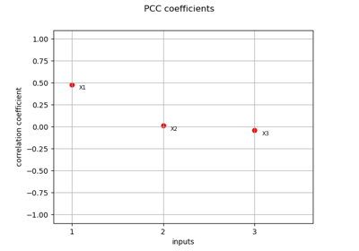
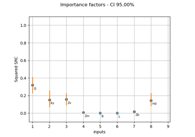
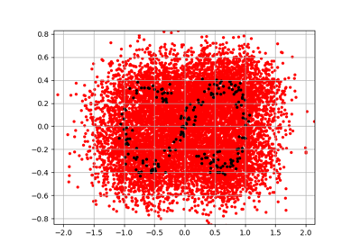
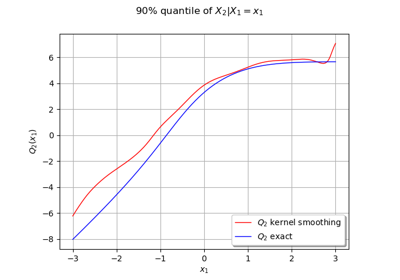


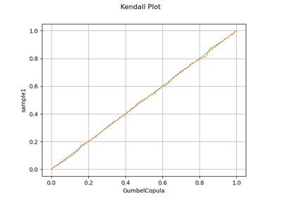
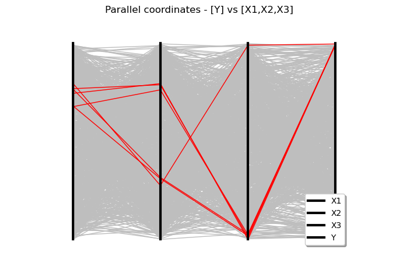

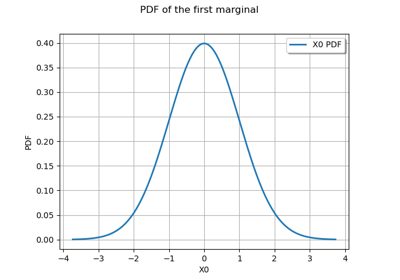

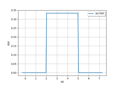
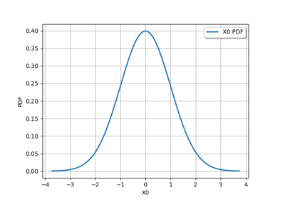
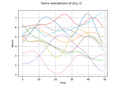
Create a process from random vectors and processes


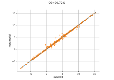
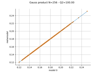
Create a polynomial chaos metamodel by integration on the cantilever beam

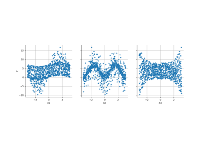
Create a polynomial chaos for the Ishigami function: a quick start guide to polynomial chaos
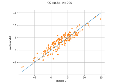
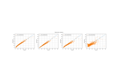
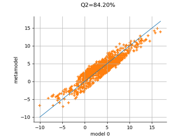
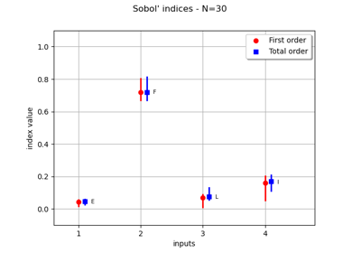
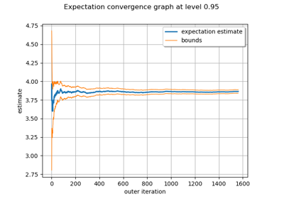
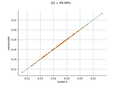

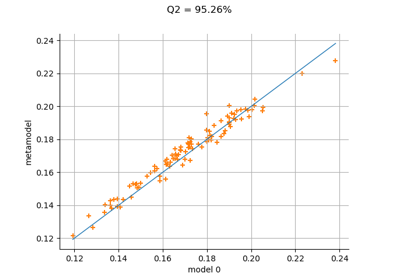
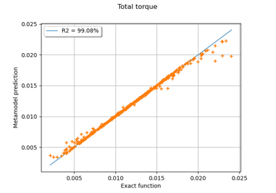
Example of multi output Kriging on the fire satellite model
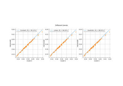
Kriging: choose a polynomial trend on the beam model
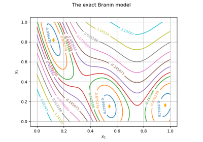

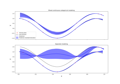
Kriging: metamodel with continuous and categorical variables
Evaluate the mean of a random vector by simulations


Use the Adaptive Directional Stratification Algorithm

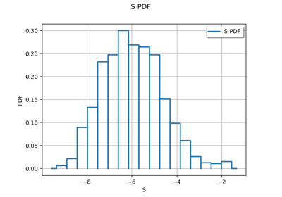
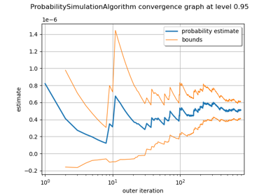
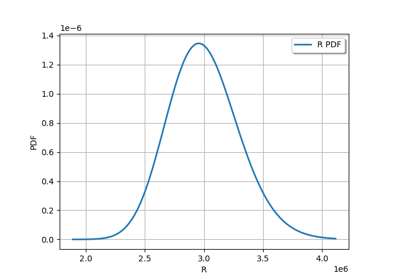
Estimate a probability with Monte-Carlo on axial stressed beam: a quick start guide to reliability
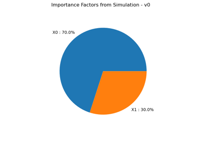

Axial stressed beam : comparing different methods to estimate a probability
An illustrated example of a FORM probability estimate
Using the FORM - SORM algorithms on a nonlinear function
Estimate Sobol indices on a field to point function
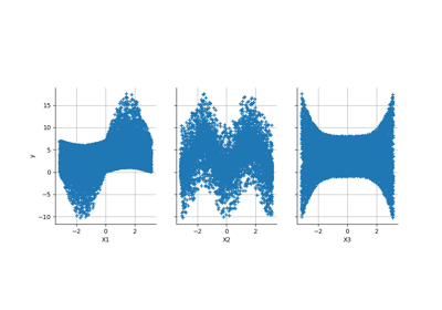
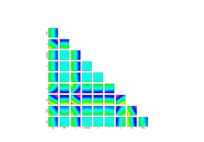
Example of sensitivity analyses on the wing weight model
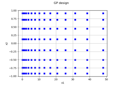
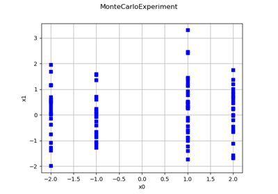
Create a design of experiments with discrete and continuous variables
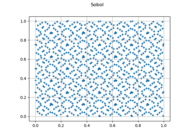
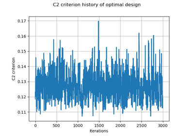
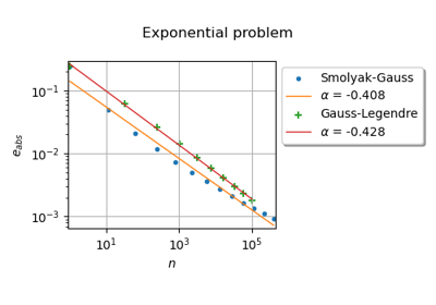

Defining Python and symbolic functions: a quick start introduction to functions
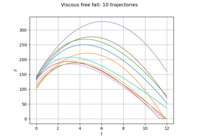
Define a function with a field output: the viscous free fall example
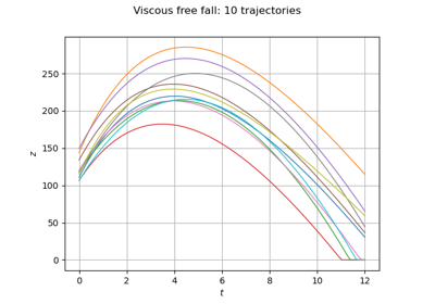
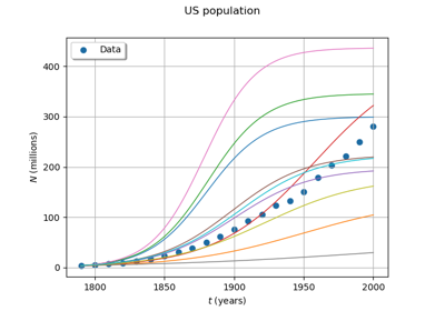
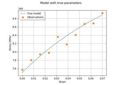
Generate observations of the Chaboche mechanical model
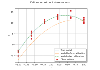
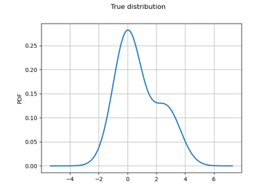
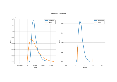
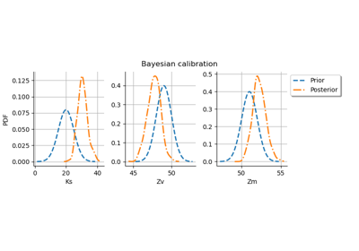
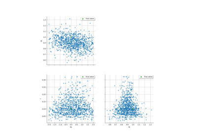
Linear Regression with interval-censored observations
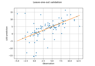
Compute leave-one-out error of a polynomial chaos expansion


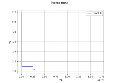
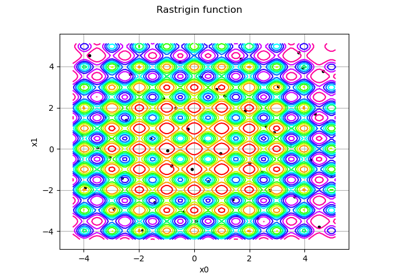
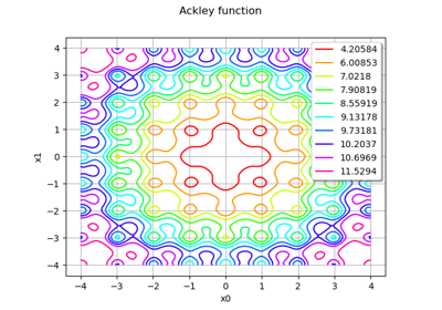
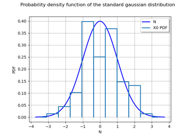
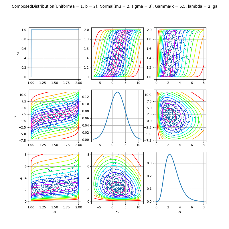