PersistentObject
- class PersistentObject(*args, **kwargs)
PersistentObject saves and reloads the object’s internal state.
Methods
Accessor to the object's name.
getName()Accessor to the object's name.
hasName()Test if the object is named.
setName(name)Accessor to the object's name.
- __init__(*args, **kwargs)
- getClassName()
Accessor to the object’s name.
- Returns:
- class_namestr
The object class name (object.__class__.__name__).
- getName()
Accessor to the object’s name.
- Returns:
- namestr
The name of the object.
- hasName()
Test if the object is named.
- Returns:
- hasNamebool
True if the name is not empty.
- setName(name)
Accessor to the object’s name.
- Parameters:
- namestr
The name of the object.
Examples using the class


A quick start guide to the Point and Sample classes


Fitting a distribution with customized maximum likelihood


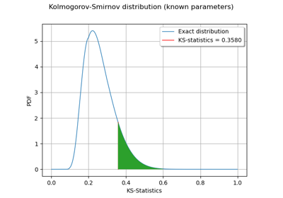
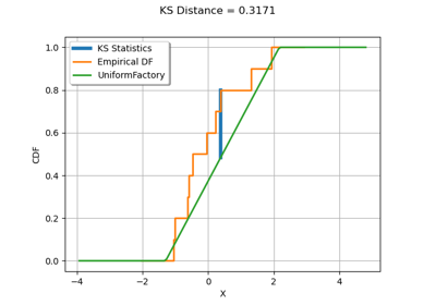
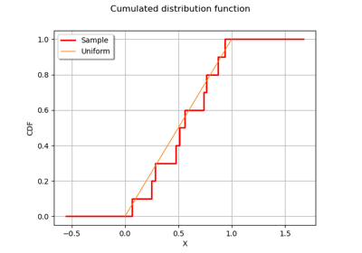
Kolmogorov-Smirnov : get the statistics distribution
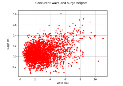
Estimate tail dependence coefficients on the wave-surge data
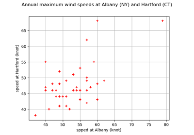
Estimate tail dependence coefficients on the wind data


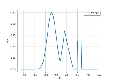
Create the distribution of the maximum of independent distributions
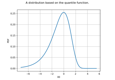
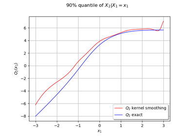
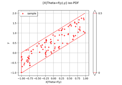
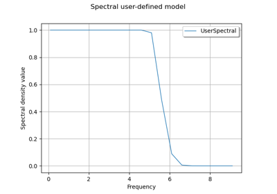
Create your own distribution given its quantile function


Create a gaussian process from a cov. model using HMatrix
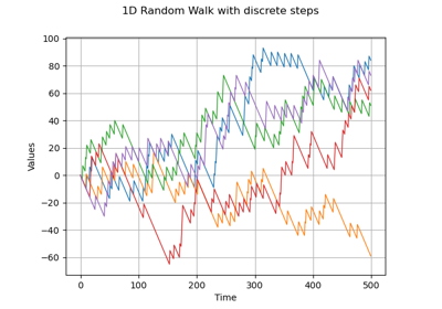

Create a process from random vectors and processes
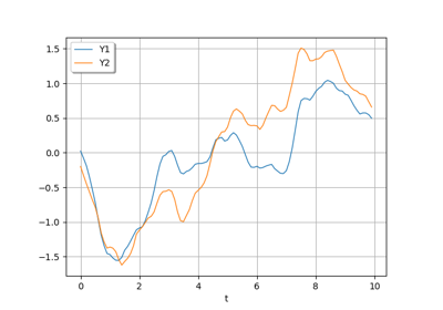
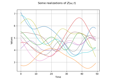
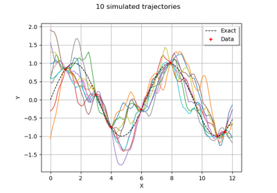
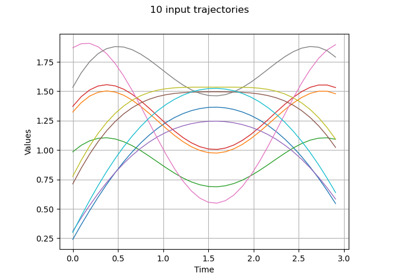
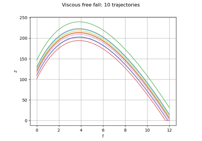
Sample trajectories from a Gaussian Process with correlated outputs

Apply a transform or inverse transform on your polynomial chaos


Create a full or sparse polynomial chaos expansion
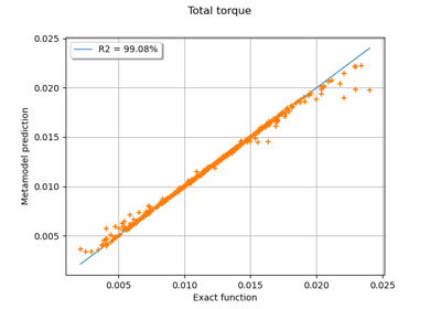
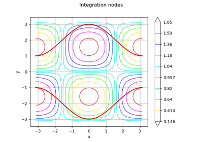
Create a polynomial chaos metamodel by integration on the cantilever beam

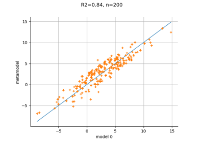
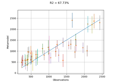
Create a polynomial chaos metamodel from a data set
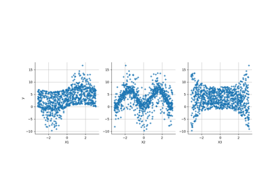
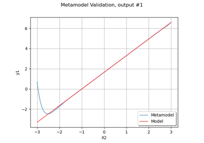
Create a polynomial chaos for the Ishigami function: a quick start guide to polynomial chaos

Example of multi output Kriging on the fire satellite model
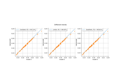
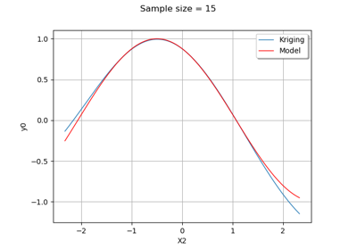
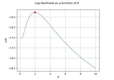
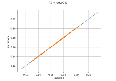
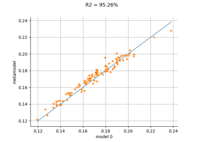
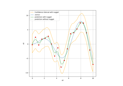
Kriging: choose a polynomial trend on the beam model

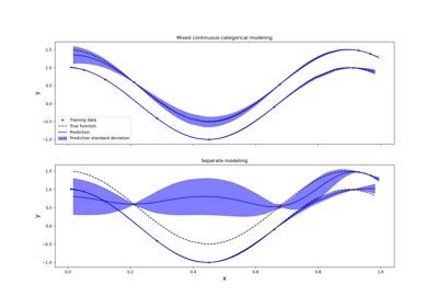
Kriging: metamodel with continuous and categorical variables
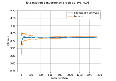
Evaluate the mean of a random vector by simulations


Use the Adaptive Directional Stratification Algorithm

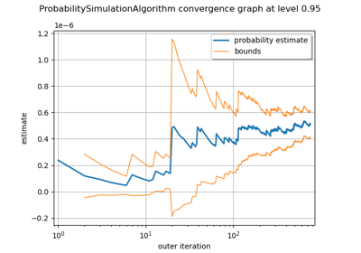
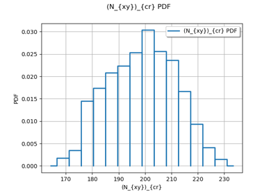
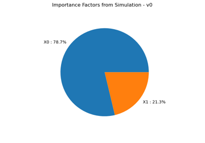
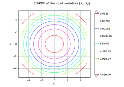
Use the post-analytical importance sampling algorithm


Estimate a probability with Monte-Carlo on axial stressed beam: a quick start guide to reliability
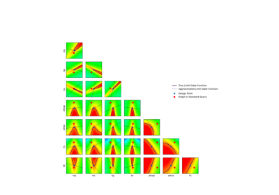
Use the FORM algorithm in case of several design points
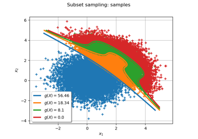
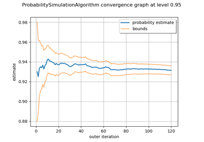
Non parametric Adaptive Importance Sampling (NAIS)

Test the design point with the Strong Maximum Test

Axial stressed beam : comparing different methods to estimate a probability
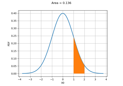
An illustrated example of a FORM probability estimate
Using the FORM - SORM algorithms on a nonlinear function

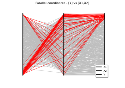
Estimate Sobol indices on a field to point function
Sobol’ sensitivity indices using rank-based algorithm
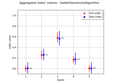
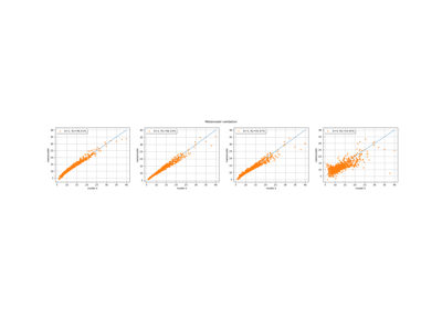
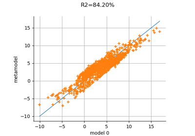
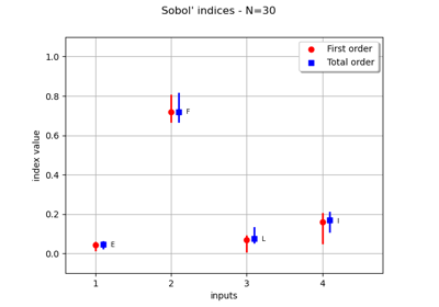
Estimate Sobol’ indices for a function with multivariate output
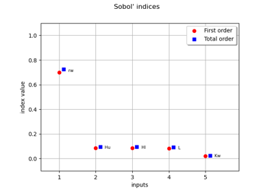
Example of sensitivity analyses on the wing weight model

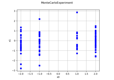
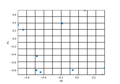
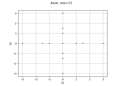
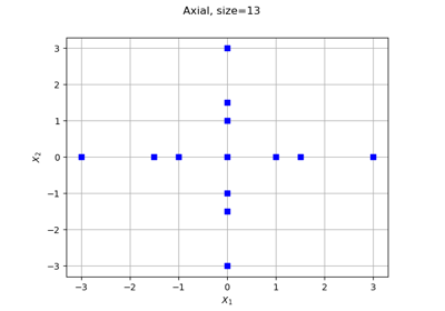
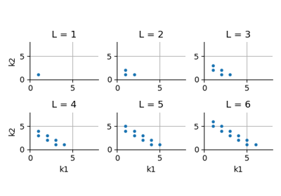
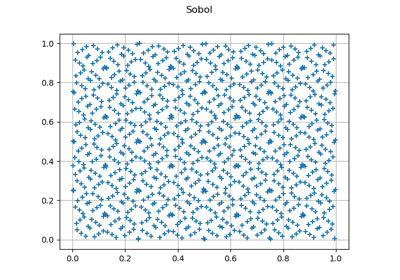
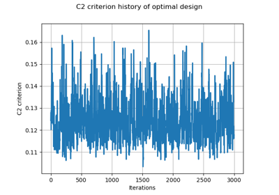
Create mixed deterministic and probabilistic designs of experiments
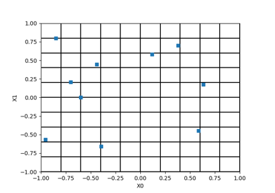
Create a design of experiments with discrete and continuous variables


Defining Python and symbolic functions: a quick start introduction to functions


Create a multivariate basis of functions from scalar multivariable functions


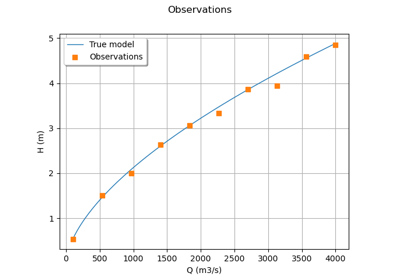
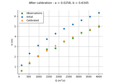
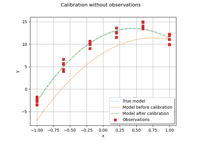
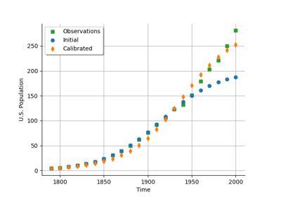
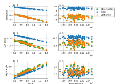
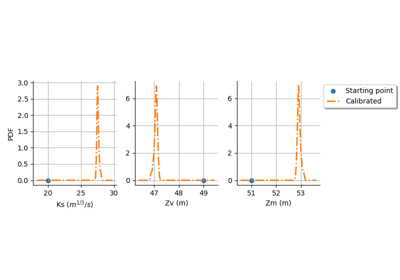
Calibrate a parametric model: a quick-start guide to calibration
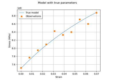
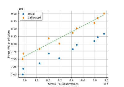
Generate observations of the Chaboche mechanical model

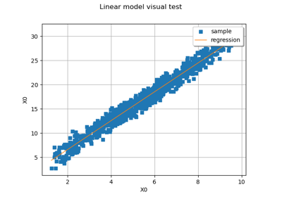
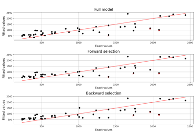
Linear Regression with interval-censored observations


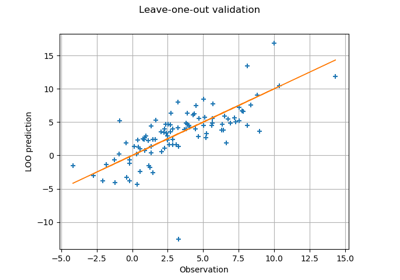
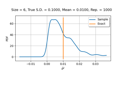
Compute leave-one-out error of a polynomial chaos expansion
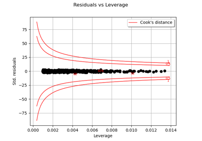
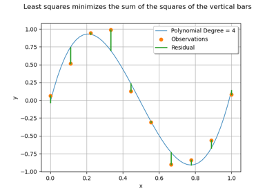
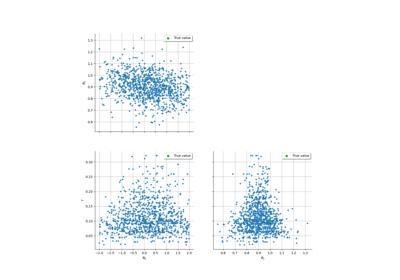
Compute confidence intervals of a regression model from data
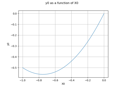
Compute confidence intervals of a univariate noisy function


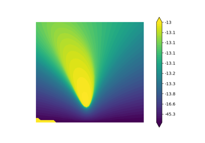
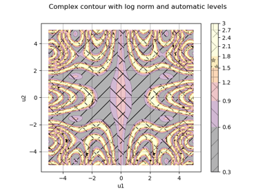
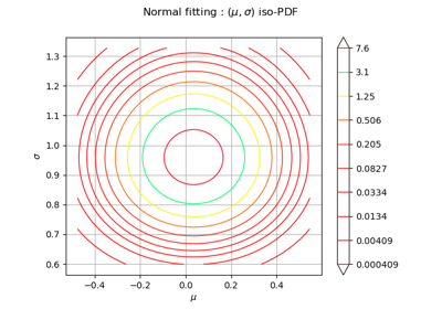
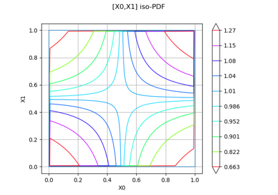
Plot the log-likelihood contours of a distribution